Money and death
We return to the death penalty.
import numpy as np
import pandas as pd
import matplotlib.pyplot as plt
%matplotlib inline
# Make plots look a little bit more fancy
plt.style.use('fivethirtyeight')
In this case, we are going to analyze whether people with higher incomes are more likely to favor the death penalty.
To do this, we are going to analyze the results from a sample of the US General Social Survey from 2002.
If you are running on your laptop, download the data file GSS2002.csv.
# Read the data into a data frame
gss = pd.read_csv('GSS2002.csv')
gss
| ID | Region | Gender | Race | Education | Marital | Religion | Happy | Income | PolParty | ... | Marijuana | DeathPenalty | OwnGun | GunLaw | SpendMilitary | SpendEduc | SpendEnv | SpendSci | Pres00 | Postlife | |
|---|---|---|---|---|---|---|---|---|---|---|---|---|---|---|---|---|---|---|---|---|---|
| 0 | 1 | South Central | Female | White | HS | Divorced | Inter-nondenominational | Pretty happy | 30000-34999 | Strong Rep | ... | NaN | Favor | No | Favor | Too little | Too little | About right | About right | Bush | Yes |
| 1 | 2 | South Central | Male | White | Bachelors | Married | Protestant | Pretty happy | 75000-89999 | Not Str Rep | ... | Not legal | Favor | Yes | Oppose | About right | Too little | About right | About right | Bush | Yes |
| 2 | 3 | South Central | Female | White | HS | Separated | Protestant | NaN | 35000-39999 | Strong Rep | ... | NaN | NaN | NaN | NaN | NaN | NaN | NaN | NaN | Bush | NaN |
| 3 | 4 | South Central | Female | White | Left HS | Divorced | Protestant | NaN | 50000-59999 | Ind, Near Dem | ... | NaN | NaN | NaN | NaN | About right | Too little | Too little | Too little | NaN | NaN |
| 4 | 5 | South Central | Male | White | Left HS | Divorced | Protestant | NaN | 40000-49999 | Ind | ... | NaN | NaN | NaN | NaN | NaN | NaN | NaN | NaN | NaN | NaN |
| 5 | 6 | South Central | Male | White | HS | Divorced | Catholic | Pretty happy | 40000-49999 | Ind, Near Rep | ... | NaN | Favor | Yes | Oppose | Too little | Too little | Too little | Too little | Bush | Yes |
| 6 | 7 | South Central | Female | White | Bachelors | Married | Protestant | NaN | NaN | Strong Rep | ... | NaN | NaN | NaN | NaN | NaN | NaN | NaN | NaN | Bush | NaN |
| 7 | 8 | South Central | Female | White | HS | Married | Protestant | NaN | NaN | Ind | ... | NaN | NaN | NaN | NaN | Too little | Too little | About right | About right | Bush | NaN |
| 8 | 9 | South Central | Male | White | HS | Divorced | Catholic | Not too happy | 60000-74999 | Strong Rep | ... | Legal | Favor | Yes | Oppose | NaN | NaN | NaN | NaN | Bush | Yes |
| 9 | 10 | South Central | Female | Other | HS | Never Married | Catholic | NaN | under 1000 | Ind, Near Rep | ... | NaN | NaN | NaN | NaN | Too much | Too little | Too little | Too little | NaN | NaN |
| 10 | 11 | South Central | Male | White | HS | Married | None | NaN | 50000-59999 | Strong Rep | ... | NaN | NaN | NaN | NaN | NaN | NaN | NaN | NaN | NaN | NaN |
| 11 | 12 | South Central | Male | White | Left HS | Married | Protestant | NaN | 110000-129999 | Not Str Rep | ... | NaN | NaN | NaN | NaN | About right | About right | Too much | Too much | Bush | NaN |
| 12 | 13 | South Central | Male | Black | Graduate | Married | Catholic | NaN | 90000-109999 | Not Str Dem | ... | NaN | NaN | NaN | NaN | Too much | About right | Too little | About right | NaN | NaN |
| 13 | 14 | South Central | Female | White | HS | Divorced | Protestant | Pretty happy | 10000-124999 | Strong Rep | ... | Not legal | Favor | No | Favor | NaN | NaN | NaN | NaN | Bush | Yes |
| 14 | 15 | South Central | Female | Other | HS | Married | Moslem/Islam | NaN | NaN | Ind, Near Rep | ... | NaN | NaN | NaN | NaN | About right | Too much | Too much | Too much | NaN | NaN |
| 15 | 16 | South Central | Female | White | HS | Married | Orthodox-Christian | NaN | NaN | Ind | ... | NaN | NaN | NaN | NaN | NaN | NaN | NaN | NaN | NaN | NaN |
| 16 | 17 | South Central | Female | White | HS | Divorced | Christian | Not too happy | NaN | Not Str Rep | ... | NaN | Favor | No | Favor | About right | Too little | Too little | About right | NaN | Yes |
| 17 | 18 | South Central | Male | White | HS | Never Married | Protestant | Very happy | 40000-49999 | Strong Rep | ... | Legal | Favor | NaN | NaN | NaN | NaN | NaN | NaN | Bush | Yes |
| 18 | 19 | South Central | Male | White | Jr Col | Divorced | None | Pretty happy | 75000-89999 | Ind, Near Dem | ... | Legal | Favor | Yes | Oppose | Too little | About right | Too much | About right | NaN | NaN |
| 19 | 20 | South Central | Male | White | HS | Never Married | None | NaN | 25000-29999 | Other party | ... | NaN | NaN | NaN | NaN | NaN | NaN | NaN | NaN | Nader | NaN |
| 20 | 21 | South Central | Female | Black | HS | Never Married | Protestant | NaN | 25000-29999 | Ind | ... | NaN | NaN | NaN | NaN | NaN | NaN | NaN | NaN | NaN | NaN |
| 21 | 22 | South Central | Male | Black | HS | Separated | Catholic | Pretty happy | 17500-19999 | Not Str Dem | ... | NaN | Oppose | No | Favor | About right | Too little | Too little | About right | NaN | Yes |
| 22 | 23 | South Central | Male | Other | Bachelors | Married | Moslem/Islam | Not too happy | 50000-59999 | Not Str Dem | ... | Legal | Favor | NaN | NaN | NaN | NaN | NaN | NaN | Gore | Yes |
| 23 | 24 | South Central | Female | Black | HS | Married | Protestant | NaN | 40000-49999 | Not Str Dem | ... | NaN | NaN | NaN | NaN | NaN | NaN | NaN | NaN | Gore | NaN |
| 24 | 25 | South Central | Male | White | HS | Married | Protestant | NaN | 40000-49999 | Strong Rep | ... | NaN | NaN | NaN | NaN | NaN | NaN | NaN | NaN | Bush | NaN |
| 25 | 26 | South Central | Female | White | HS | Widowed | Protestant | NaN | NaN | Other party | ... | NaN | NaN | NaN | NaN | Too little | Too little | About right | About right | Bush | NaN |
| 26 | 27 | South Central | Female | White | HS | Widowed | Catholic | Pretty happy | NaN | Other party | ... | NaN | Favor | No | Favor | NaN | NaN | NaN | NaN | Bush | Yes |
| 27 | 28 | South Central | Female | Other | Bachelors | Divorced | None | NaN | 25000-29999 | Ind, Near Dem | ... | NaN | NaN | NaN | NaN | Too much | Too little | Too little | Too little | NaN | NaN |
| 28 | 29 | South Central | Female | Other | HS | Never Married | Catholic | NaN | 1000-2999 | Ind | ... | NaN | NaN | NaN | NaN | NaN | NaN | NaN | NaN | NaN | NaN |
| 29 | 30 | South Central | Female | White | HS | Never Married | Protestant | NaN | 10000-124999 | Ind | ... | NaN | NaN | NaN | NaN | About right | NaN | About right | NaN | NaN | NaN |
| ... | ... | ... | ... | ... | ... | ... | ... | ... | ... | ... | ... | ... | ... | ... | ... | ... | ... | ... | ... | ... | ... |
| 2735 | 2736 | South Atlantic | Male | White | Graduate | Married | Protestant | Pretty happy | NaN | Strong Rep | ... | Not legal | Favor | Yes | Favor | Too little | Too much | Too much | Too little | Bush | Yes |
| 2736 | 2737 | South Atlantic | Female | White | Bachelors | Married | Protestant | NaN | 25000-29999 | Strong Rep | ... | NaN | NaN | NaN | NaN | NaN | NaN | NaN | NaN | Bush | NaN |
| 2737 | 2738 | South Atlantic | Female | Black | HS | Married | Protestant | Pretty happy | 60000-74999 | Strong Dem | ... | Not legal | Oppose | NaN | NaN | NaN | NaN | NaN | NaN | Gore | Yes |
| 2738 | 2739 | South Atlantic | Female | White | HS | Widowed | Protestant | Pretty happy | 25000-29999 | Strong Dem | ... | Legal | NaN | No | Favor | NaN | Too little | Too little | About right | Gore | Yes |
| 2739 | 2740 | South Atlantic | Female | White | Left HS | Separated | Protestant | NaN | NaN | Strong Rep | ... | NaN | NaN | NaN | NaN | NaN | NaN | NaN | NaN | Bush | NaN |
| 2740 | 2741 | South Atlantic | Female | White | Bachelors | Separated | Protestant | NaN | NaN | Ind, Near Rep | ... | NaN | NaN | NaN | NaN | NaN | NaN | NaN | NaN | Bush | NaN |
| 2741 | 2742 | South Atlantic | Male | White | HS | Married | Protestant | Pretty happy | 15000-17499 | Not Str Rep | ... | NaN | Favor | Yes | Favor | NaN | NaN | NaN | NaN | Bush | Yes |
| 2742 | 2743 | South Atlantic | Male | White | HS | Never Married | Protestant | Pretty happy | 25000-29999 | Ind, Near Rep | ... | Legal | Favor | NaN | NaN | Too little | Too little | Too little | Too little | Bush | Yes |
| 2743 | 2744 | South Atlantic | Male | Black | HS | Married | Protestant | NaN | 22500-24999 | Strong Dem | ... | NaN | NaN | NaN | NaN | NaN | NaN | NaN | NaN | NaN | NaN |
| 2744 | 2745 | South Atlantic | Male | White | HS | Never Married | Protestant | NaN | NaN | Ind, Near Rep | ... | NaN | NaN | NaN | NaN | About right | Too little | About right | Too little | NaN | NaN |
| 2745 | 2746 | Pacific | Female | White | Bachelors | Married | Protestant | Pretty happy | NaN | Not Str Rep | ... | NaN | Favor | No | Favor | NaN | NaN | NaN | NaN | Bush | NaN |
| 2746 | 2747 | Pacific | Female | White | HS | Widowed | Catholic | Pretty happy | NaN | Strong Rep | ... | Not legal | Oppose | NaN | NaN | Too little | Too little | Too much | Too little | Bush | Yes |
| 2747 | 2748 | Pacific | Female | White | HS | Never Married | Protestant | Very happy | 8000-9999 | Not Str Rep | ... | NaN | Favor | Yes | Favor | NaN | NaN | NaN | NaN | NaN | Yes |
| 2748 | 2749 | Pacific | Female | White | HS | Widowed | Protestant | NaN | NaN | Not Str Dem | ... | NaN | NaN | NaN | NaN | Too little | Too little | Too much | About right | Gore | NaN |
| 2749 | 2750 | Mid-Atl | Male | White | Jr Col | Married | Protestant | NaN | 22500-24999 | Not Str Rep | ... | NaN | NaN | NaN | NaN | NaN | NaN | NaN | NaN | Bush | NaN |
| 2750 | 2751 | Mid-Atl | Female | White | HS | Married | Protestant | Not too happy | 6000-6999 | Ind | ... | Not legal | NaN | NaN | NaN | NaN | NaN | NaN | NaN | Gore | Yes |
| 2751 | 2752 | Mid-Atl | Male | White | Left HS | Married | Protestant | NaN | 22500-24999 | Strong Rep | ... | NaN | NaN | NaN | NaN | Too little | Too little | Too little | About right | NaN | NaN |
| 2752 | 2753 | South Central | Female | White | Jr Col | Married | Protestant | NaN | NaN | Other party | ... | NaN | NaN | NaN | NaN | NaN | NaN | NaN | NaN | NaN | NaN |
| 2753 | 2754 | South Central | Male | Black | HS | Never Married | Catholic | Very happy | 35000-39999 | Not Str Dem | ... | NaN | Favor | No | Favor | About right | Too little | Too little | Too little | Bush | NaN |
| 2754 | 2755 | South Central | Female | White | HS | Divorced | Protestant | NaN | NaN | Strong Rep | ... | NaN | NaN | NaN | NaN | About right | About right | Too little | About right | Bush | NaN |
| 2755 | 2756 | South Central | Female | White | HS | Married | Protestant | NaN | 35000-39999 | Not Str Dem | ... | NaN | NaN | NaN | NaN | NaN | NaN | NaN | NaN | Bush | NaN |
| 2756 | 2757 | South Central | Male | Black | HS | Married | Protestant | Very happy | 30000-34999 | Strong Dem | ... | Not legal | Favor | No | Favor | NaN | NaN | NaN | NaN | Gore | Yes |
| 2757 | 2758 | New Engl | Male | White | HS | Divorced | Protestant | NaN | 6000-6999 | Not Str Rep | ... | NaN | NaN | NaN | NaN | NaN | NaN | NaN | NaN | NaN | NaN |
| 2758 | 2759 | New Engl | Female | White | HS | Never Married | None | NaN | 12500-14999 | Ind, Near Dem | ... | NaN | NaN | NaN | NaN | NaN | NaN | NaN | NaN | Gore | NaN |
| 2759 | 2760 | New Engl | Female | White | HS | Divorced | None | NaN | 20000-22499 | Not Str Rep | ... | NaN | NaN | NaN | NaN | Too much | About right | Too little | NaN | NaN | NaN |
| 2760 | 2761 | New Engl | Male | White | Left HS | Never Married | None | Pretty happy | 22500-24999 | Ind, Near Dem | ... | Legal | Favor | NaN | NaN | NaN | NaN | NaN | NaN | NaN | Yes |
| 2761 | 2762 | New Engl | Male | White | Bachelors | Married | None | NaN | NaN | Ind, Near Dem | ... | NaN | NaN | NaN | NaN | NaN | NaN | NaN | NaN | Nader | NaN |
| 2762 | 2763 | New Engl | Female | White | HS | Married | Catholic | NaN | NaN | Not Str Rep | ... | NaN | NaN | NaN | NaN | Too little | Too much | Too much | About right | Bush | NaN |
| 2763 | 2764 | South Atlantic | Male | Black | HS | Never Married | Protestant | NaN | NaN | Ind | ... | NaN | NaN | NaN | NaN | About right | Too little | Too little | Too much | NaN | NaN |
| 2764 | 2765 | South Atlantic | Male | White | HS | Married | Protestant | Very happy | 60000-74999 | Not Str Rep | ... | Legal | Oppose | Yes | Favor | NaN | NaN | NaN | NaN | Bush | Yes |
2765 rows × 21 columns
Each row corresponds to a single respondent.
Show the column names:
gss.columns
Index(['ID', 'Region', 'Gender', 'Race', 'Education', 'Marital', 'Religion',
       'Happy', 'Income', 'PolParty', 'Politics', 'Marijuana', 'DeathPenalty',
       'OwnGun', 'GunLaw', 'SpendMilitary', 'SpendEduc', 'SpendEnv',
       'SpendSci', 'Pres00', 'Postlife'],
      dtype='object')
We want to work with only two columns from this data frame. These are “Income”, and “DeathPenalty”.
“Income” gives the income bracket of the respondent. “DeathPenalty” is the answer to a question about whether they “Favor” or “Oppose” the death penalty.
First make a list with the names of the columns that we want.
cols = ['Income', 'DeathPenalty']
cols
['Income', 'DeathPenalty']
Next make a new data frame by indexing the data frame with this list.
The new data frame has only the columns we selected.
money_death = gss[cols]
money_death
| Income | DeathPenalty | |
|---|---|---|
| 0 | 30000-34999 | Favor |
| 1 | 75000-89999 | Favor |
| 2 | 35000-39999 | NaN |
| 3 | 50000-59999 | NaN |
| 4 | 40000-49999 | NaN |
| 5 | 40000-49999 | Favor |
| 6 | NaN | NaN |
| 7 | NaN | NaN |
| 8 | 60000-74999 | Favor |
| 9 | under 1000 | NaN |
| 10 | 50000-59999 | NaN |
| 11 | 110000-129999 | NaN |
| 12 | 90000-109999 | NaN |
| 13 | 10000-124999 | Favor |
| 14 | NaN | NaN |
| 15 | NaN | NaN |
| 16 | NaN | Favor |
| 17 | 40000-49999 | Favor |
| 18 | 75000-89999 | Favor |
| 19 | 25000-29999 | NaN |
| 20 | 25000-29999 | NaN |
| 21 | 17500-19999 | Oppose |
| 22 | 50000-59999 | Favor |
| 23 | 40000-49999 | NaN |
| 24 | 40000-49999 | NaN |
| 25 | NaN | NaN |
| 26 | NaN | Favor |
| 27 | 25000-29999 | NaN |
| 28 | 1000-2999 | NaN |
| 29 | 10000-124999 | NaN |
| ... | ... | ... |
| 2735 | NaN | Favor |
| 2736 | 25000-29999 | NaN |
| 2737 | 60000-74999 | Oppose |
| 2738 | 25000-29999 | NaN |
| 2739 | NaN | NaN |
| 2740 | NaN | NaN |
| 2741 | 15000-17499 | Favor |
| 2742 | 25000-29999 | Favor |
| 2743 | 22500-24999 | NaN |
| 2744 | NaN | NaN |
| 2745 | NaN | Favor |
| 2746 | NaN | Oppose |
| 2747 | 8000-9999 | Favor |
| 2748 | NaN | NaN |
| 2749 | 22500-24999 | NaN |
| 2750 | 6000-6999 | NaN |
| 2751 | 22500-24999 | NaN |
| 2752 | NaN | NaN |
| 2753 | 35000-39999 | Favor |
| 2754 | NaN | NaN |
| 2755 | 35000-39999 | NaN |
| 2756 | 30000-34999 | Favor |
| 2757 | 6000-6999 | NaN |
| 2758 | 12500-14999 | NaN |
| 2759 | 20000-22499 | NaN |
| 2760 | 22500-24999 | Favor |
| 2761 | NaN | NaN |
| 2762 | NaN | NaN |
| 2763 | NaN | NaN |
| 2764 | 60000-74999 | Oppose |
2765 rows × 2 columns
There are many missing question responses, indicated by NaN. To
make our life easier, we drop the respondents who didn’t specify an
income bracket, and those who did not give an answer to the death penalty
question. We use Pandas dropna method of the data frame, to drop all rows
that have any missing values in the row.
money_death = money_death.dropna()
money_death
| Income | DeathPenalty | |
|---|---|---|
| 0 | 30000-34999 | Favor |
| 1 | 75000-89999 | Favor |
| 5 | 40000-49999 | Favor |
| 8 | 60000-74999 | Favor |
| 13 | 10000-124999 | Favor |
| 17 | 40000-49999 | Favor |
| 18 | 75000-89999 | Favor |
| 21 | 17500-19999 | Oppose |
| 22 | 50000-59999 | Favor |
| 31 | 30000-34999 | Favor |
| 32 | 50000-59999 | Oppose |
| 33 | 75000-89999 | Oppose |
| 35 | under 1000 | Oppose |
| 36 | 7000-7999 | Oppose |
| 37 | 60000-74999 | Favor |
| 42 | 30000-34999 | Favor |
| 45 | 35000-39999 | Favor |
| 46 | under 1000 | Favor |
| 52 | 17500-19999 | Favor |
| 55 | 35000-39999 | Favor |
| 58 | 1000-2999 | Favor |
| 62 | 50000-59999 | Favor |
| 64 | 12500-14999 | Favor |
| 74 | 110000-129999 | Oppose |
| 77 | 75000-89999 | Favor |
| 78 | 35000-39999 | Favor |
| 81 | 30000-34999 | Favor |
| 92 | 20000-22499 | Favor |
| 93 | 60000-74999 | Favor |
| 95 | 60000-74999 | Oppose |
| ... | ... | ... |
| 2671 | 75000-89999 | Favor |
| 2677 | 1000-2999 | Oppose |
| 2678 | 15000-17499 | Favor |
| 2684 | under 1000 | Favor |
| 2689 | 3000-3999 | Favor |
| 2690 | 22500-24999 | Oppose |
| 2692 | 8000-9999 | Favor |
| 2696 | 3000-3999 | Oppose |
| 2697 | 30000-34999 | Favor |
| 2699 | 25000-29999 | Favor |
| 2702 | 8000-9999 | Oppose |
| 2706 | 10000-124999 | Oppose |
| 2709 | 12500-14999 | Oppose |
| 2714 | 12500-14999 | Favor |
| 2715 | 40000-49999 | Favor |
| 2716 | 130000-149999 | Favor |
| 2717 | 3000-3999 | Oppose |
| 2723 | 22500-24999 | Favor |
| 2725 | 40000-49999 | Favor |
| 2726 | 15000-17499 | Oppose |
| 2727 | 12500-14999 | Favor |
| 2729 | under 1000 | Favor |
| 2737 | 60000-74999 | Oppose |
| 2741 | 15000-17499 | Favor |
| 2742 | 25000-29999 | Favor |
| 2747 | 8000-9999 | Favor |
| 2753 | 35000-39999 | Favor |
| 2756 | 30000-34999 | Favor |
| 2760 | 22500-24999 | Favor |
| 2764 | 60000-74999 | Oppose |
904 rows × 2 columns
Get the income column.
income = money_death['Income']
Show the unique values:
income.value_counts()
40000-49999      88
30000-34999      78
50000-59999      72
25000-29999      60
35000-39999      54
60000-74999      51
20000-22499      44
12500-14999      44
130000-149999    43
22500-24999      40
110000-129999    38
17500-19999      37
15000-17499      36
10000-124999     36
1000-2999        32
8000-9999        32
75000-89999      26
3000-3999        19
under 1000       17
5000-5999        16
4000-4999        13
90000-109999     11
7000-7999         9
6000-6999         8
Name: Income, dtype: int64
These are strings. We want to get income as a number. We estimate this by recoding the “Income” column. We replace the string, giving the income bracket, with the average of the minimum and maximum in the range.
We can do this with a recoder function. We have not covered functions yet, so do not worry about the details of this function.
def recode_income(value):
    if value == 'under 1000':
        return 500
    low_str, high_str = value.split('-')
    low, high = int(low_str), int(high_str)
    return np.mean([low, high])
Here is what the recoder function gives with the lowest income bracket.
recode_income('under 1000')
500
Here is the return from a higher bracket:
recode_income('90000-109999')
99999.5
Use this function to recode the “Income” strings into numbers. Again, we have not covered the apply method yet, so don’t worry about the details.
income_ish = income.apply(recode_income)
income_ish
0        32499.5
1        82499.5
5        44999.5
8        67499.5
13       67499.5
17       44999.5
18       82499.5
21       18749.5
22       54999.5
31       32499.5
32       54999.5
33       82499.5
35         500.0
36        7499.5
37       67499.5
42       32499.5
45       37499.5
46         500.0
52       18749.5
55       37499.5
58        1999.5
62       54999.5
64       13749.5
74      119999.5
77       82499.5
78       37499.5
81       32499.5
92       21249.5
93       67499.5
95       67499.5
          ...
2671     82499.5
2677      1999.5
2678     16249.5
2684       500.0
2689      3499.5
2690     23749.5
2692      8999.5
2696      3499.5
2697     32499.5
2699     27499.5
2702      8999.5
2706     67499.5
2709     13749.5
2714     13749.5
2715     44999.5
2716    139999.5
2717      3499.5
2723     23749.5
2725     44999.5
2726     16249.5
2727     13749.5
2729       500.0
2737     67499.5
2741     16249.5
2742     27499.5
2747      8999.5
2753     37499.5
2756     32499.5
2760     23749.5
2764     67499.5
Name: Income, Length: 904, dtype: float64
Now get the results of the answer to the death penalty question.
death = money_death['DeathPenalty']
death.value_counts()
Favor     622
Oppose    282
Name: DeathPenalty, dtype: int64
We will identify the rows for respondents who are in favor of the death penalty. To do this, we make a Boolean vector:
death == 'Favor'
0        True
1        True
5        True
8        True
13       True
17       True
18       True
21      False
22       True
31       True
32      False
33      False
35      False
36      False
37       True
42       True
45       True
46       True
52       True
55       True
58       True
62       True
64       True
74      False
77       True
78       True
81       True
92       True
93       True
95      False
        ...
2671     True
2677    False
2678     True
2684     True
2689     True
2690    False
2692     True
2696    False
2697     True
2699     True
2702    False
2706    False
2709    False
2714     True
2715     True
2716     True
2717    False
2723     True
2725     True
2726    False
2727     True
2729     True
2737    False
2741     True
2742     True
2747     True
2753     True
2756     True
2760     True
2764    False
Name: DeathPenalty, Length: 904, dtype: bool
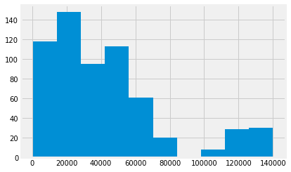
Use this vector to select the income values for the respondents in favor of the death penalty. Show the distribution of values.
favor_income = income_ish[death == 'Favor']
favor_income.hist();
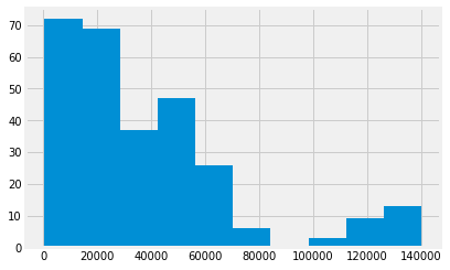
Likewise select incomes for those opposed. Show the distribution.
oppose_income = income_ish[death == 'Oppose']
oppose_income.hist();
Calculate the difference in mean income between the groups. This is the difference we observe.
actual_diff = np.mean(favor_income) - np.mean(oppose_income)
actual_diff
4535.163012246019
We want to know whether this difference in income is compatible with random sampling. That is, we want to know whether a difference this large is plausible, if the incomes are in fact random samples from the same population.
To estimate how variable the mean differences can be, for such random sampling, we simulate this sampling by pooling the income values that we have, from the two groups, and the permuting them.
First, we get the number of respondents in favor of the death penalty.
n_favor = len(favor_income)
n_favor
622
Then we pool the in-favor and oppose groups.
pooled = np.append(favor_income, oppose_income)
To do the random sampling we permute the values, so the pooled vector is
a random mixture of the two groups.
np.random.shuffle(pooled)
Treat the first n_favor observations from this shuffled vector as
our simulated in-favor group. The rest are our simulated oppose
group.
fake_favor = pooled[:n_favor]
fake_oppose = pooled[n_favor:]
Calculate the difference in means for this simulation.
fake_diff = np.mean(fake_favor) - np.mean(fake_oppose)
fake_diff
3143.6351793573704
Now it is your turn. Do this simulation 10000 times, to build up the distribution of differences compatible with random sampling.
Use the Brexit ages notebook for inspiration.
differences = np.zeros(10000)
for i in np.arange(10000):
    # Permute the pooled incomes
    np.random.shuffle(pooled)
    # Make a fake favor sample

    # Make a fake opposed sample

    # Calculate the mean difference for the fake samples

    # Put the mean difference into the differences array.
When you have that working, do a histogram of the differences.
# Your code here
You can get an idea of where the actual difference we saw sits on this histogram, and therefore how likely that difference is, assuming the incomes come from the same underlying population of incomes.
To be more specific, count how many of the differences you calculated were greater than or equal to the actual difference.
# Your code here
Now calculate the proportion of these differences, to give an estimate of the probability of seeing a difference this large, if the incomes all come from the same underlying population:
# Your code here