4.1 Introduction to data frames
Introduction to data frames
Start by loading the usual plotting libraries.
import numpy as np
import matplotlib.pyplot as plt
%matplotlib inline
# Make plots look a little bit more fancy
plt.style.use('fivethirtyeight')
Pandas is a Python package that implements data frames, and functions that operate on data frames.
import pandas as pd
Data frames and series
We start by loading data from a Comma Separated Value file (CSV file). If you are running on your laptop, you should download the gender_stats.csv file to the same directory as this notebook.
# Load the data file
gender_data = pd.read_csv('gender_stats.csv')
This is our usual assignment statement. The LHS is gender_data, the variable name. The RHS is an expression, that returns a value.
What type of value does it return?
type(gender_data)
pandas.core.frame.DataFrame
Pandas integrates with the Notebook, so, if you display a data frame in the notebook, it does a nice display of rows and columns.
gender_data
| country | fert_rate | gdp | health_exp_per_cap | health_exp_pub | prim_ed_girls | mat_mort_ratio | population | |
|---|---|---|---|---|---|---|---|---|
| 0 | Afghanistan | 4.954500 | 1.996102e+10 | 161.138034 | 2.834598 | 40.109708 | 444.00 | 3.271584e+07 |
| 1 | Albania | 1.769250 | 1.232759e+10 | 574.202694 | 2.836021 | 47.201082 | 29.25 | 2.888280e+06 |
| 2 | Algeria | 2.866000 | 1.907346e+11 | 870.766508 | 4.984252 | 47.675617 | 142.50 | 3.909906e+07 |
| 3 | American Samoa | NaN | 6.405000e+08 | NaN | NaN | NaN | NaN | 5.542200e+04 |
| 4 | Andorra | NaN | 3.197538e+09 | 4421.224933 | 7.260281 | 47.123345 | NaN | 7.954740e+04 |
| 5 | Angola | 6.123000 | 1.119365e+11 | 254.747970 | 2.447546 | NaN | 501.25 | 2.693754e+07 |
| 6 | Antigua and Barbuda | 2.082000 | 1.298213e+09 | 1152.493656 | 3.676514 | 48.291463 | NaN | 9.887240e+04 |
| 7 | Arab World | 3.397587 | 2.709059e+12 | 761.401727 | 2.873840 | 47.119776 | 161.00 | 3.899620e+08 |
| 8 | Argentina | 2.328000 | 5.509810e+11 | 1148.256142 | 2.782216 | 48.915810 | 53.75 | 4.297667e+07 |
| 9 | Armenia | 1.545500 | 1.088536e+10 | 348.663884 | 1.916016 | 46.782180 | 27.25 | 2.904683e+06 |
| 10 | Aruba | 1.663250 | NaN | NaN | NaN | 48.721939 | NaN | 1.037444e+05 |
| 11 | Australia | 1.861500 | 1.422994e+12 | 4256.058988 | 6.292381 | 48.576707 | 6.00 | 2.344456e+07 |
| 12 | Austria | 1.455000 | 4.074943e+11 | 4930.298893 | 8.504276 | 48.556078 | 4.00 | 8.566294e+06 |
| 13 | Azerbaijan | 1.980000 | 6.200300e+10 | 956.709718 | 1.197249 | 46.157363 | 25.25 | 9.531856e+06 |
| 14 | Bahamas, The | 1.877250 | 8.688000e+09 | 1727.128385 | 3.308626 | NaN | 81.50 | 3.819036e+05 |
| 15 | Bahrain | 2.065250 | 3.200401e+10 | 2030.158316 | 2.976386 | 49.116838 | 15.25 | 1.349810e+06 |
| 16 | Bangladesh | 2.193250 | 1.745451e+11 | 85.968844 | 0.860447 | 50.460564 | 194.75 | 1.593712e+08 |
| 17 | Barbados | 1.792250 | 4.413080e+09 | 1062.840088 | 4.828680 | 48.878181 | 28.00 | 2.833384e+05 |
| 18 | Belarus | 1.677000 | 6.478294e+10 | 986.236757 | 3.876601 | 48.685741 | 4.00 | 9.480348e+06 |
| 19 | Belgium | 1.755000 | 4.942218e+11 | 4297.838005 | 8.221003 | 48.864675 | 7.00 | 1.122850e+07 |
| 20 | Belize | 2.594750 | 1.680325e+09 | 471.967465 | 3.744844 | 48.317238 | 29.25 | 3.517636e+05 |
| 21 | Benin | 4.806750 | 8.778151e+09 | 83.726190 | 2.206916 | 47.211127 | 417.50 | 1.029371e+07 |
| 22 | Bermuda | 1.617500 | 5.555624e+09 | NaN | NaN | 48.423588 | NaN | 6.510080e+04 |
| 23 | Bhutan | 2.061250 | 1.975145e+09 | 277.526670 | 2.706908 | 49.572296 | 161.75 | 7.759054e+05 |
| 24 | Bolivia | 2.995250 | 3.150932e+10 | 381.007594 | 4.192031 | 48.464175 | 218.25 | 1.056280e+07 |
| 25 | Bosnia and Herzegovina | 1.267000 | 1.732333e+10 | 941.504655 | 6.841021 | 48.634905 | 11.75 | 3.574396e+06 |
| 26 | Botswana | 2.845000 | 1.511339e+10 | 880.909202 | 3.552071 | 48.844009 | 138.75 | 2.169170e+06 |
| 27 | Brazil | 1.795250 | 2.198766e+12 | 1303.199104 | 3.773473 | 47.784577 | 49.50 | 2.041595e+08 |
| 28 | British Virgin Islands | NaN | NaN | NaN | NaN | 47.581520 | NaN | 2.958540e+04 |
| 29 | Brunei Darussalam | 1.884000 | 1.571922e+10 | 1795.924160 | 2.335194 | 48.523699 | 23.75 | 4.115812e+05 |
| ... | ... | ... | ... | ... | ... | ... | ... | ... |
| 233 | Syrian Arab Republic | 2.967750 | NaN | 269.945739 | 1.507166 | 48.047394 | 62.00 | 1.931967e+07 |
| 234 | Tajikistan | 3.495750 | 8.036228e+09 | 169.745970 | 1.976367 | 48.260680 | 33.25 | 8.363844e+06 |
| 235 | Tanzania | 5.181250 | 4.493554e+10 | 131.704162 | 2.648609 | 50.666580 | 429.50 | 5.228132e+07 |
| 236 | Thailand | 1.516750 | 4.061369e+11 | 581.927487 | 3.183842 | 48.213034 | 21.00 | 6.838499e+07 |
| 237 | Timor-Leste | 5.797750 | 1.361430e+09 | 98.577296 | 1.140440 | 48.337367 | 240.25 | 1.212718e+06 |
| 238 | Togo | 4.620000 | 4.183610e+09 | 71.263825 | 2.037809 | 48.270471 | 380.75 | 7.230904e+06 |
| 239 | Tonga | 3.745750 | 4.391789e+08 | 250.962504 | 3.987285 | 47.697931 | 129.25 | 1.059094e+05 |
| 240 | Trinidad and Tobago | 1.782750 | 2.457095e+10 | 1778.148073 | 3.071370 | NaN | 63.25 | 1.353877e+06 |
| 241 | Tunisia | 2.140000 | 4.482437e+10 | 782.950522 | 4.118771 | 48.142132 | 63.25 | 1.114441e+07 |
| 242 | Turkey | 2.078000 | 8.951756e+11 | 997.374772 | 4.189521 | 48.789477 | 17.50 | 7.703435e+07 |
| 243 | Turkmenistan | 2.313750 | 3.797310e+10 | 288.572644 | 1.349303 | 48.906879 | 43.50 | 5.465637e+06 |
| 244 | Turks and Caicos Islands | NaN | NaN | NaN | NaN | 48.846884 | NaN | 3.370340e+04 |
| 245 | Tuvalu | NaN | 3.646999e+07 | 563.500592 | 15.506929 | 47.472414 | NaN | 1.091000e+04 |
| 246 | Uganda | 5.822500 | 2.594146e+10 | 132.892684 | 2.014349 | 50.099485 | 366.50 | 3.886534e+07 |
| 247 | Ukraine | 1.510250 | 1.353793e+11 | 628.579254 | 3.960185 | 48.984198 | 24.25 | 4.530270e+07 |
| 248 | United Arab Emirates | 1.793000 | 3.750271e+11 | 2202.407569 | 2.581168 | 48.789260 | 6.00 | 9.080299e+06 |
| 249 | United Kingdom | 1.842500 | 2.768864e+12 | 3357.983675 | 7.720655 | 48.791809 | 9.25 | 6.464156e+07 |
| 250 | United States | 1.860875 | 1.736912e+13 | 9060.068657 | 8.121961 | 48.758830 | 14.00 | 3.185582e+08 |
| 251 | Upper middle income | 1.795244 | 2.097441e+13 | 870.897512 | 3.358153 | 47.112001 | 43.25 | 2.540966e+09 |
| 252 | Uruguay | 2.027000 | 5.434513e+10 | 1721.507752 | 6.044403 | 48.295555 | 15.50 | 3.419977e+06 |
| 253 | Uzbekistan | 2.372750 | 6.134065e+10 | 334.476754 | 3.118842 | 48.387434 | 37.00 | 3.078450e+07 |
| 254 | Vanuatu | 3.364750 | 7.828760e+08 | 125.568712 | 3.689874 | 47.301617 | 82.50 | 2.588964e+05 |
| 255 | Venezuela, RB | 2.378250 | 3.761463e+11 | 896.815314 | 1.587088 | 48.400934 | 97.00 | 3.073452e+07 |
| 256 | Vietnam | 1.959500 | 1.818207e+11 | 368.374550 | 3.779501 | 48.021053 | 54.75 | 9.074240e+07 |
| 257 | Virgin Islands (U.S.) | 1.760000 | 3.812000e+09 | NaN | NaN | NaN | NaN | 1.041414e+05 |
| 258 | West Bank and Gaza | 4.208000 | 1.250822e+10 | NaN | NaN | 48.828520 | 47.50 | 4.296960e+06 |
| 259 | World | 2.464282 | 7.613006e+13 | 1223.941243 | 5.947058 | 48.076575 | 223.75 | 7.269321e+09 |
| 260 | Yemen, Rep. | 4.225750 | 3.681934e+10 | 207.949700 | 1.417836 | 44.470076 | 399.75 | 2.624661e+07 |
| 261 | Zambia | 5.394250 | 2.428099e+10 | 185.556359 | 2.687290 | 49.934484 | 233.75 | 1.563322e+07 |
| 262 | Zimbabwe | 3.943000 | 1.549551e+10 | 115.519881 | 2.695188 | 49.529875 | 398.00 | 1.542096e+07 |
263 rows × 8 columns
The data frame has rows and columns. Like other Python objects, it has attributes. These are pieces of data associated with the data frame. You have already seen methods, which are functions associated with the data frame. You can access attributes in the same way as you access methods, by typing the variable name, followed by a dot ., followed by the attribute name.
For example, one attribute of the data frame, is the shape:
gender_data.shape
(263, 8)
Another attribute is columns. This has the column names. For
example, here is a good way of quickly seeing the column names
for a data frame:
gender_data.columns
Index(['country', 'fert_rate', 'gdp', 'health_exp_per_cap', 'health_exp_pub',
       'prim_ed_girls', 'mat_mort_ratio', 'population'],
      dtype='object')
You need more information about what these column names refer to. Here are the longer descriptions from the original data source (link above):
fert_rate: Fertility rate, total (births per woman).gdp: GDP (current US$).health_exp_per_cap: Health expenditure per capita, PPP (constant 2011 international \$).health_exp_pub: Health expenditure, public (% of GDP).prim_ed_girls: Primary education, pupils (% female).mat_mort_ratio: Maternal mortality ratio (modeled estimate, per 100,000 live births).population: Population, total.
You have just seen array slicing (in Selecting with arrays. You remember that array slicing uses square brackets. Data frames also allow slicing. For example, we often want to get all the data for a single column of the data frame. To do this, we use the same square bracket notation as we use for array slicing, with the name of the column inside the square brackets.
gdp = gender_data['gdp']
What type of thing is this column of data?
type(gdp)
pandas.core.series.Series
Here are the values for gdp. You will notice that these are
the same values you saw in the “gdp” column when you displayed
the whole data frame.
gdp
0      1.996102e+10
1      1.232759e+10
2      1.907346e+11
3      6.405000e+08
4      3.197538e+09
5      1.119365e+11
6      1.298213e+09
7      2.709059e+12
8      5.509810e+11
9      1.088536e+10
10              NaN
11     1.422994e+12
12     4.074943e+11
13     6.200300e+10
14     8.688000e+09
15     3.200401e+10
16     1.745451e+11
17     4.413080e+09
18     6.478294e+10
19     4.942218e+11
20     1.680325e+09
21     8.778151e+09
22     5.555624e+09
23     1.975145e+09
24     3.150932e+10
25     1.732333e+10
26     1.511339e+10
27     2.198766e+12
28              NaN
29     1.571922e+10
           ...
233             NaN
234    8.036228e+09
235    4.493554e+10
236    4.061369e+11
237    1.361430e+09
238    4.183610e+09
239    4.391789e+08
240    2.457095e+10
241    4.482437e+10
242    8.951756e+11
243    3.797310e+10
244             NaN
245    3.646999e+07
246    2.594146e+10
247    1.353793e+11
248    3.750271e+11
249    2.768864e+12
250    1.736912e+13
251    2.097441e+13
252    5.434513e+10
253    6.134065e+10
254    7.828760e+08
255    3.761463e+11
256    1.818207e+11
257    3.812000e+09
258    1.250822e+10
259    7.613006e+13
260    3.681934e+10
261    2.428099e+10
262    1.549551e+10
Name: gdp, Length: 263, dtype: float64
What are these values like 6.405000e+08? These are numbers,
in scientific
notation.
Scientific notation is a compact way of writing very large or
very small numbers. The value after e above is the
exponent, in this case 08. The number above means $6.405
- 10^8$. For example, here is $2 * 10^7$:
2e7
20000000.0
Missing values and NaN
Looking at the values of gdp (and therefore, the values of the
gdp column of gender_data, we see that some of the values
are NaN, which means Not a Number. Pandas uses this marker to
indicate values that are not available, or missing data.
Numpy does not like to calculate with NaN values. Here is Numpy trying to calculate the median of the gdp values.
np.median(gdp)
nan
Notice the warning about an invalid value.
Numpy recognizes that one or more values are NaN and refuses to guess what to do, when calculating the median.
You saw from the shape above that gender_data has 263 rows. We can use the general Python len function, to see how many elements there are in gdp.
len(gdp)
263
As expected, it has the same number of elements as there are rows in gender_data.
The count method of the series gives the number of values that are not missing - that is - not NaN.
gdp.count()
246
Plotting with methods
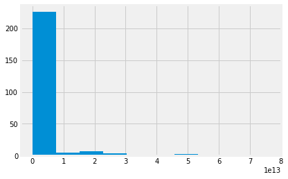
The gdp variable is a sequence of values, so we can do a histogram on these values, as we have done histograms on arrays.
plt.hist(gdp);

Notice the multiple warnings as Matplotlib tried to calculate the bin widths for the histogram. These are from the NaN values.
Another way to do the histogram, is to use the hist method of the series.
A method is a function attached to a value. In this case hist is a function attached to a value of type Series.
Using the hist method instead of the plt.hist function can make the code a bit easier to read. The method also has the advantage that it discards the NaN values, by default, so it does not generate the same warnings.
gdp.hist();
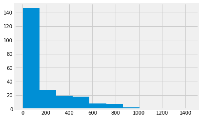
Now we have had a look at the GDP values, we will look at the
values for the mat_mort_ratio column. These are the numbers
of women who die in childbirth for every 100,000 births.
mmr = gender_data['mat_mort_ratio']
mmr
0      444.00
1       29.25
2      142.50
3         NaN
4         NaN
5      501.25
6         NaN
7      161.00
8       53.75
9       27.25
10        NaN
11       6.00
12       4.00
13      25.25
14      81.50
15      15.25
16     194.75
17      28.00
18       4.00
19       7.00
20      29.25
21     417.50
22        NaN
23     161.75
24     218.25
25      11.75
26     138.75
27      49.50
28        NaN
29      23.75
        ...
233     62.00
234     33.25
235    429.50
236     21.00
237    240.25
238    380.75
239    129.25
240     63.25
241     63.25
242     17.50
243     43.50
244       NaN
245       NaN
246    366.50
247     24.25
248      6.00
249      9.25
250     14.00
251     43.25
252     15.50
253     37.00
254     82.50
255     97.00
256     54.75
257       NaN
258     47.50
259    223.75
260    399.75
261    233.75
262    398.00
Name: mat_mort_ratio, Length: 263, dtype: float64
mmr.hist();
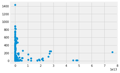
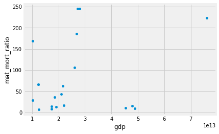
We are interested in the relationship of gpp and mmr. Maybe richer countries have better health care, and fewer maternal deaths.
Here is a plot, using the standard Matplotlib scatter
function.
plt.scatter(gdp, mmr);
We can do the same plot using the plot.scatter method on the data frame. In that case, we specify the column names that should go on the x and the y axes.
gender_data.plot.scatter('gdp', 'mat_mort_ratio');
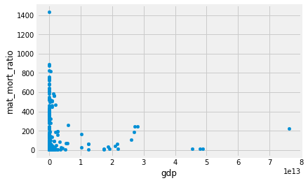
An advantage of doing it this way is that we get the column names on the x and y axes by default.
Showing the top 5 values with the head method
We have already seen that Pandas will display the data frame with nice formatting. If the data frame is long, it will display only the first few and the last few rows:
gender_data
| country | fert_rate | gdp | health_exp_per_cap | health_exp_pub | prim_ed_girls | mat_mort_ratio | population | |
|---|---|---|---|---|---|---|---|---|
| 0 | Afghanistan | 4.954500 | 1.996102e+10 | 161.138034 | 2.834598 | 40.109708 | 444.00 | 3.271584e+07 |
| 1 | Albania | 1.769250 | 1.232759e+10 | 574.202694 | 2.836021 | 47.201082 | 29.25 | 2.888280e+06 |
| 2 | Algeria | 2.866000 | 1.907346e+11 | 870.766508 | 4.984252 | 47.675617 | 142.50 | 3.909906e+07 |
| 3 | American Samoa | NaN | 6.405000e+08 | NaN | NaN | NaN | NaN | 5.542200e+04 |
| 4 | Andorra | NaN | 3.197538e+09 | 4421.224933 | 7.260281 | 47.123345 | NaN | 7.954740e+04 |
| 5 | Angola | 6.123000 | 1.119365e+11 | 254.747970 | 2.447546 | NaN | 501.25 | 2.693754e+07 |
| 6 | Antigua and Barbuda | 2.082000 | 1.298213e+09 | 1152.493656 | 3.676514 | 48.291463 | NaN | 9.887240e+04 |
| 7 | Arab World | 3.397587 | 2.709059e+12 | 761.401727 | 2.873840 | 47.119776 | 161.00 | 3.899620e+08 |
| 8 | Argentina | 2.328000 | 5.509810e+11 | 1148.256142 | 2.782216 | 48.915810 | 53.75 | 4.297667e+07 |
| 9 | Armenia | 1.545500 | 1.088536e+10 | 348.663884 | 1.916016 | 46.782180 | 27.25 | 2.904683e+06 |
| 10 | Aruba | 1.663250 | NaN | NaN | NaN | 48.721939 | NaN | 1.037444e+05 |
| 11 | Australia | 1.861500 | 1.422994e+12 | 4256.058988 | 6.292381 | 48.576707 | 6.00 | 2.344456e+07 |
| 12 | Austria | 1.455000 | 4.074943e+11 | 4930.298893 | 8.504276 | 48.556078 | 4.00 | 8.566294e+06 |
| 13 | Azerbaijan | 1.980000 | 6.200300e+10 | 956.709718 | 1.197249 | 46.157363 | 25.25 | 9.531856e+06 |
| 14 | Bahamas, The | 1.877250 | 8.688000e+09 | 1727.128385 | 3.308626 | NaN | 81.50 | 3.819036e+05 |
| 15 | Bahrain | 2.065250 | 3.200401e+10 | 2030.158316 | 2.976386 | 49.116838 | 15.25 | 1.349810e+06 |
| 16 | Bangladesh | 2.193250 | 1.745451e+11 | 85.968844 | 0.860447 | 50.460564 | 194.75 | 1.593712e+08 |
| 17 | Barbados | 1.792250 | 4.413080e+09 | 1062.840088 | 4.828680 | 48.878181 | 28.00 | 2.833384e+05 |
| 18 | Belarus | 1.677000 | 6.478294e+10 | 986.236757 | 3.876601 | 48.685741 | 4.00 | 9.480348e+06 |
| 19 | Belgium | 1.755000 | 4.942218e+11 | 4297.838005 | 8.221003 | 48.864675 | 7.00 | 1.122850e+07 |
| 20 | Belize | 2.594750 | 1.680325e+09 | 471.967465 | 3.744844 | 48.317238 | 29.25 | 3.517636e+05 |
| 21 | Benin | 4.806750 | 8.778151e+09 | 83.726190 | 2.206916 | 47.211127 | 417.50 | 1.029371e+07 |
| 22 | Bermuda | 1.617500 | 5.555624e+09 | NaN | NaN | 48.423588 | NaN | 6.510080e+04 |
| 23 | Bhutan | 2.061250 | 1.975145e+09 | 277.526670 | 2.706908 | 49.572296 | 161.75 | 7.759054e+05 |
| 24 | Bolivia | 2.995250 | 3.150932e+10 | 381.007594 | 4.192031 | 48.464175 | 218.25 | 1.056280e+07 |
| 25 | Bosnia and Herzegovina | 1.267000 | 1.732333e+10 | 941.504655 | 6.841021 | 48.634905 | 11.75 | 3.574396e+06 |
| 26 | Botswana | 2.845000 | 1.511339e+10 | 880.909202 | 3.552071 | 48.844009 | 138.75 | 2.169170e+06 |
| 27 | Brazil | 1.795250 | 2.198766e+12 | 1303.199104 | 3.773473 | 47.784577 | 49.50 | 2.041595e+08 |
| 28 | British Virgin Islands | NaN | NaN | NaN | NaN | 47.581520 | NaN | 2.958540e+04 |
| 29 | Brunei Darussalam | 1.884000 | 1.571922e+10 | 1795.924160 | 2.335194 | 48.523699 | 23.75 | 4.115812e+05 |
| ... | ... | ... | ... | ... | ... | ... | ... | ... |
| 233 | Syrian Arab Republic | 2.967750 | NaN | 269.945739 | 1.507166 | 48.047394 | 62.00 | 1.931967e+07 |
| 234 | Tajikistan | 3.495750 | 8.036228e+09 | 169.745970 | 1.976367 | 48.260680 | 33.25 | 8.363844e+06 |
| 235 | Tanzania | 5.181250 | 4.493554e+10 | 131.704162 | 2.648609 | 50.666580 | 429.50 | 5.228132e+07 |
| 236 | Thailand | 1.516750 | 4.061369e+11 | 581.927487 | 3.183842 | 48.213034 | 21.00 | 6.838499e+07 |
| 237 | Timor-Leste | 5.797750 | 1.361430e+09 | 98.577296 | 1.140440 | 48.337367 | 240.25 | 1.212718e+06 |
| 238 | Togo | 4.620000 | 4.183610e+09 | 71.263825 | 2.037809 | 48.270471 | 380.75 | 7.230904e+06 |
| 239 | Tonga | 3.745750 | 4.391789e+08 | 250.962504 | 3.987285 | 47.697931 | 129.25 | 1.059094e+05 |
| 240 | Trinidad and Tobago | 1.782750 | 2.457095e+10 | 1778.148073 | 3.071370 | NaN | 63.25 | 1.353877e+06 |
| 241 | Tunisia | 2.140000 | 4.482437e+10 | 782.950522 | 4.118771 | 48.142132 | 63.25 | 1.114441e+07 |
| 242 | Turkey | 2.078000 | 8.951756e+11 | 997.374772 | 4.189521 | 48.789477 | 17.50 | 7.703435e+07 |
| 243 | Turkmenistan | 2.313750 | 3.797310e+10 | 288.572644 | 1.349303 | 48.906879 | 43.50 | 5.465637e+06 |
| 244 | Turks and Caicos Islands | NaN | NaN | NaN | NaN | 48.846884 | NaN | 3.370340e+04 |
| 245 | Tuvalu | NaN | 3.646999e+07 | 563.500592 | 15.506929 | 47.472414 | NaN | 1.091000e+04 |
| 246 | Uganda | 5.822500 | 2.594146e+10 | 132.892684 | 2.014349 | 50.099485 | 366.50 | 3.886534e+07 |
| 247 | Ukraine | 1.510250 | 1.353793e+11 | 628.579254 | 3.960185 | 48.984198 | 24.25 | 4.530270e+07 |
| 248 | United Arab Emirates | 1.793000 | 3.750271e+11 | 2202.407569 | 2.581168 | 48.789260 | 6.00 | 9.080299e+06 |
| 249 | United Kingdom | 1.842500 | 2.768864e+12 | 3357.983675 | 7.720655 | 48.791809 | 9.25 | 6.464156e+07 |
| 250 | United States | 1.860875 | 1.736912e+13 | 9060.068657 | 8.121961 | 48.758830 | 14.00 | 3.185582e+08 |
| 251 | Upper middle income | 1.795244 | 2.097441e+13 | 870.897512 | 3.358153 | 47.112001 | 43.25 | 2.540966e+09 |
| 252 | Uruguay | 2.027000 | 5.434513e+10 | 1721.507752 | 6.044403 | 48.295555 | 15.50 | 3.419977e+06 |
| 253 | Uzbekistan | 2.372750 | 6.134065e+10 | 334.476754 | 3.118842 | 48.387434 | 37.00 | 3.078450e+07 |
| 254 | Vanuatu | 3.364750 | 7.828760e+08 | 125.568712 | 3.689874 | 47.301617 | 82.50 | 2.588964e+05 |
| 255 | Venezuela, RB | 2.378250 | 3.761463e+11 | 896.815314 | 1.587088 | 48.400934 | 97.00 | 3.073452e+07 |
| 256 | Vietnam | 1.959500 | 1.818207e+11 | 368.374550 | 3.779501 | 48.021053 | 54.75 | 9.074240e+07 |
| 257 | Virgin Islands (U.S.) | 1.760000 | 3.812000e+09 | NaN | NaN | NaN | NaN | 1.041414e+05 |
| 258 | West Bank and Gaza | 4.208000 | 1.250822e+10 | NaN | NaN | 48.828520 | 47.50 | 4.296960e+06 |
| 259 | World | 2.464282 | 7.613006e+13 | 1223.941243 | 5.947058 | 48.076575 | 223.75 | 7.269321e+09 |
| 260 | Yemen, Rep. | 4.225750 | 3.681934e+10 | 207.949700 | 1.417836 | 44.470076 | 399.75 | 2.624661e+07 |
| 261 | Zambia | 5.394250 | 2.428099e+10 | 185.556359 | 2.687290 | 49.934484 | 233.75 | 1.563322e+07 |
| 262 | Zimbabwe | 3.943000 | 1.549551e+10 | 115.519881 | 2.695188 | 49.529875 | 398.00 | 1.542096e+07 |
263 rows × 8 columns
Notice the ... in the center of this listing, to show that it has not printed some rows.
Sometimes we do not want to see all these rows, but only - say - the top five rows. The head method of the data frame is a useful way to do this:
gender_data.head()
| country | fert_rate | gdp | health_exp_per_cap | health_exp_pub | prim_ed_girls | mat_mort_ratio | population | |
|---|---|---|---|---|---|---|---|---|
| 0 | Afghanistan | 4.95450 | 1.996102e+10 | 161.138034 | 2.834598 | 40.109708 | 444.00 | 32715838.4 |
| 1 | Albania | 1.76925 | 1.232759e+10 | 574.202694 | 2.836021 | 47.201082 | 29.25 | 2888280.2 |
| 2 | Algeria | 2.86600 | 1.907346e+11 | 870.766508 | 4.984252 | 47.675617 | 142.50 | 39099060.4 |
| 3 | American Samoa | NaN | 6.405000e+08 | NaN | NaN | NaN | NaN | 55422.0 |
| 4 | Andorra | NaN | 3.197538e+09 | 4421.224933 | 7.260281 | 47.123345 | NaN | 79547.4 |
The Series also has a head method, that does the same thing:
gdp.head()
0    1.996102e+10
1    1.232759e+10
2    1.907346e+11
3    6.405000e+08
4    3.197538e+09
Name: gdp, dtype: float64
Selecting rows
We often want to select rows from the data frame that match some criterion.
Say we want to select the rows corresponding the countries with a high GDP.
Looking at the histogram of gdp above, we could try this as a threshold to identify high GDP countries.
high_gdp = gdp > 1e13
high_gdp
0      False
1      False
2      False
3      False
4      False
5      False
6      False
7      False
8      False
9      False
10     False
11     False
12     False
13     False
14     False
15     False
16     False
17     False
18     False
19     False
20     False
21     False
22     False
23     False
24     False
25     False
26     False
27     False
28     False
29     False
       ...
233    False
234    False
235    False
236    False
237    False
238    False
239    False
240    False
241    False
242    False
243    False
244    False
245    False
246    False
247    False
248    False
249    False
250     True
251     True
252    False
253    False
254    False
255    False
256    False
257    False
258    False
259     True
260    False
261    False
262    False
Name: gdp, Length: 263, dtype: bool
type(high_gdp)
pandas.core.series.Series
Notice that high_gdp is a Boolean series, like the Boolean arrays you have already seen. It has True for elements corresponding to countries with gdp value greater than 1e13 and False otherwise.
We can use this Boolean series to select rows from the data frame. The loc attribute of the data frame allows us to LOCate values in the data frame. For our Boolean series, it works like this:
rich_gender_data = gender_data.loc[high_gdp]
rich_gender_data
| country | fert_rate | gdp | health_exp_per_cap | health_exp_pub | prim_ed_girls | mat_mort_ratio | population | |
|---|---|---|---|---|---|---|---|---|
| 44 | China | 1.558750 | 1.018279e+13 | 657.748859 | 3.015530 | 46.297964 | 28.75 | 1.364446e+09 |
| 60 | Early-demographic dividend | 2.636376 | 1.019283e+13 | 392.428268 | 2.595967 | 48.651143 | 169.00 | 3.083697e+09 |
| 61 | East Asia & Pacific | 1.781424 | 2.168128e+13 | 835.974259 | 4.687596 | 47.212490 | 63.00 | 2.265974e+09 |
| 62 | East Asia & Pacific (IDA & IBRD) | 1.811850 | 1.239991e+13 | 558.711100 | 2.815573 | 47.098031 | 66.75 | 1.996942e+09 |
| 63 | East Asia & Pacific (excluding high income) | 1.813950 | 1.242383e+13 | 558.702327 | 2.815498 | 47.115173 | 66.75 | 2.022090e+09 |
| 71 | Euro area | 1.551004 | 1.255692e+13 | 3913.466364 | 7.956080 | 48.610030 | 6.50 | 3.384615e+08 |
| 72 | Europe & Central Asia | 1.738094 | 2.191519e+13 | 2518.566323 | 7.130694 | 48.653599 | 16.75 | 9.032073e+08 |
| 75 | European Union | 1.570012 | 1.731910e+13 | 3448.910224 | 7.816628 | 48.658777 | 8.00 | 5.082110e+08 |
| 98 | High income | 1.686585 | 4.884635e+13 | 5045.885008 | 7.602022 | 48.701030 | 10.00 | 1.175934e+09 |
| 102 | IBRD only | 2.103185 | 2.607726e+13 | 625.357428 | 3.104682 | 48.026892 | 106.25 | 4.607548e+09 |
| 103 | IDA & IBRD total | 2.587557 | 2.803020e+13 | 507.044258 | 3.013687 | 47.896337 | 244.75 | 6.113147e+09 |
| 128 | Late-demographic dividend | 1.667820 | 1.862014e+13 | 838.259199 | 3.335746 | 47.046383 | 36.00 | 2.235352e+09 |
| 140 | Low & middle income | 2.595258 | 2.724634e+13 | 498.193061 | 2.982075 | NaN | 245.25 | 6.089148e+09 |
| 160 | Middle income | 2.361746 | 2.691014e+13 | 542.340940 | 2.996480 | 48.044140 | 185.75 | 5.468296e+09 |
| 177 | North America | 1.834404 | 1.908336e+13 | 8615.535450 | 8.066182 | 48.708683 | 13.50 | 3.541404e+08 |
| 180 | OECD members | 1.749418 | 4.787743e+13 | 4566.959377 | 7.636198 | 48.704364 | 15.00 | 1.273149e+09 |
| 193 | Post-demographic dividend | 1.636470 | 4.541806e+13 | 5124.214162 | 7.858170 | 48.649863 | 10.75 | 1.092637e+09 |
| 250 | United States | 1.860875 | 1.736912e+13 | 9060.068657 | 8.121961 | 48.758830 | 14.00 | 3.185582e+08 |
| 251 | Upper middle income | 1.795244 | 2.097441e+13 | 870.897512 | 3.358153 | 47.112001 | 43.25 | 2.540966e+09 |
| 259 | World | 2.464282 | 7.613006e+13 | 1223.941243 | 5.947058 | 48.076575 | 223.75 | 7.269321e+09 |
type(rich_gender_data)
pandas.core.frame.DataFrame
rich_gender_data is a new data frame, that is a subset of the
original gender_data frame. It contains only the rows where
the GDP value is greater than 1e13 dollars. Check the display
of rich_gender_data above to confirm that the values in the
gdp column are all greater than 1e13.
We can do a scatter plot of GDP values against maternal mortality rate, and we find, oddly, that for rich countries, there is little relationship between GDP and maternal mortality.
rich_gender_data.plot.scatter('gdp', 'mat_mort_ratio')
<matplotlib.axes._subplots.AxesSubplot at 0x1178bb7b8>
Sorting data frames
Data frames have a method sort_value. This returns a new data frame with the rows sorted by the values in the column we specify.
Here are the first five rows of the original data frame:
gender_data.head()
| country | fert_rate | gdp | health_exp_per_cap | health_exp_pub | prim_ed_girls | mat_mort_ratio | population | |
|---|---|---|---|---|---|---|---|---|
| 0 | Afghanistan | 4.95450 | 1.996102e+10 | 161.138034 | 2.834598 | 40.109708 | 444.00 | 32715838.4 |
| 1 | Albania | 1.76925 | 1.232759e+10 | 574.202694 | 2.836021 | 47.201082 | 29.25 | 2888280.2 |
| 2 | Algeria | 2.86600 | 1.907346e+11 | 870.766508 | 4.984252 | 47.675617 | 142.50 | 39099060.4 |
| 3 | American Samoa | NaN | 6.405000e+08 | NaN | NaN | NaN | NaN | 55422.0 |
| 4 | Andorra | NaN | 3.197538e+09 | 4421.224933 | 7.260281 | 47.123345 | NaN | 79547.4 |
We can make a new data frame where the rows are sorted by the values in the gdp column:
gender_data_by_gdp = gender_data.sort_values('gdp')
gender_data_by_gdp.head()
| country | fert_rate | gdp | health_exp_per_cap | health_exp_pub | prim_ed_girls | mat_mort_ratio | population | |
|---|---|---|---|---|---|---|---|---|
| 245 | Tuvalu | NaN | 3.646999e+07 | 563.500592 | 15.506929 | 47.472414 | NaN | 10910.0 |
| 169 | Nauru | NaN | 1.063908e+08 | 611.020856 | 4.527932 | 49.409439 | NaN | 11695.4 |
| 121 | Kiribati | 3.74525 | 1.774306e+08 | 179.372383 | 8.279184 | 49.557255 | 95.0 | 110481.6 |
| 152 | Marshall Islands | NaN | 1.843189e+08 | 657.059335 | 14.302529 | 48.397282 | NaN | 52882.8 |
| 185 | Palau | 2.22000 | 2.548400e+08 | 1389.993077 | 6.623460 | 46.425690 | NaN | 21112.6 |
Notice that the rows are in ascending order of gdp. You can imagine, that we often want descending order. As usual you can explore how you might do this by looking at the help for the sort_values method with:
gender_data.sort_values?
in a new cell. If you do that, you discover the ascending argument, that you can use like this:
gender_data.sort_values('gdp', ascending=False)
| country | fert_rate | gdp | health_exp_per_cap | health_exp_pub | prim_ed_girls | mat_mort_ratio | population | |
|---|---|---|---|---|---|---|---|---|
| 259 | World | 2.464282 | 7.613006e+13 | 1223.941243 | 5.947058 | 48.076575 | 223.75 | 7.269321e+09 |
| 98 | High income | 1.686585 | 4.884635e+13 | 5045.885008 | 7.602022 | 48.701030 | 10.00 | 1.175934e+09 |
| 180 | OECD members | 1.749418 | 4.787743e+13 | 4566.959377 | 7.636198 | 48.704364 | 15.00 | 1.273149e+09 |
| 193 | Post-demographic dividend | 1.636470 | 4.541806e+13 | 5124.214162 | 7.858170 | 48.649863 | 10.75 | 1.092637e+09 |
| 103 | IDA & IBRD total | 2.587557 | 2.803020e+13 | 507.044258 | 3.013687 | 47.896337 | 244.75 | 6.113147e+09 |
| 140 | Low & middle income | 2.595258 | 2.724634e+13 | 498.193061 | 2.982075 | NaN | 245.25 | 6.089148e+09 |
| 160 | Middle income | 2.361746 | 2.691014e+13 | 542.340940 | 2.996480 | 48.044140 | 185.75 | 5.468296e+09 |
| 102 | IBRD only | 2.103185 | 2.607726e+13 | 625.357428 | 3.104682 | 48.026892 | 106.25 | 4.607548e+09 |
| 72 | Europe & Central Asia | 1.738094 | 2.191519e+13 | 2518.566323 | 7.130694 | 48.653599 | 16.75 | 9.032073e+08 |
| 61 | East Asia & Pacific | 1.781424 | 2.168128e+13 | 835.974259 | 4.687596 | 47.212490 | 63.00 | 2.265974e+09 |
| 251 | Upper middle income | 1.795244 | 2.097441e+13 | 870.897512 | 3.358153 | 47.112001 | 43.25 | 2.540966e+09 |
| 177 | North America | 1.834404 | 1.908336e+13 | 8615.535450 | 8.066182 | 48.708683 | 13.50 | 3.541404e+08 |
| 128 | Late-demographic dividend | 1.667820 | 1.862014e+13 | 838.259199 | 3.335746 | 47.046383 | 36.00 | 2.235352e+09 |
| 250 | United States | 1.860875 | 1.736912e+13 | 9060.068657 | 8.121961 | 48.758830 | 14.00 | 3.185582e+08 |
| 75 | European Union | 1.570012 | 1.731910e+13 | 3448.910224 | 7.816628 | 48.658777 | 8.00 | 5.082110e+08 |
| 71 | Euro area | 1.551004 | 1.255692e+13 | 3913.466364 | 7.956080 | 48.610030 | 6.50 | 3.384615e+08 |
| 63 | East Asia & Pacific (excluding high income) | 1.813950 | 1.242383e+13 | 558.702327 | 2.815498 | 47.115173 | 66.75 | 2.022090e+09 |
| 62 | East Asia & Pacific (IDA & IBRD) | 1.811850 | 1.239991e+13 | 558.711100 | 2.815573 | 47.098031 | 66.75 | 1.996942e+09 |
| 60 | Early-demographic dividend | 2.636376 | 1.019283e+13 | 392.428268 | 2.595967 | 48.651143 | 169.00 | 3.083697e+09 |
| 44 | China | 1.558750 | 1.018279e+13 | 657.748859 | 3.015530 | 46.297964 | 28.75 | 1.364446e+09 |
| 142 | Lower middle income | 2.877481 | 5.929275e+12 | 254.618642 | 1.657578 | 48.632937 | 262.50 | 2.927329e+09 |
| 129 | Latin America & Caribbean | 2.125164 | 5.845138e+12 | 1069.141865 | 3.659621 | 48.378604 | 70.75 | 6.242184e+08 |
| 130 | Latin America & Caribbean (IDA & IBRD) | 2.138122 | 5.636800e+12 | 1050.010897 | 3.585924 | 48.382980 | 71.50 | 6.080342e+08 |
| 131 | Latin America & Caribbean (excluding high income) | 2.140742 | 5.377437e+12 | 1046.116268 | 3.638974 | 48.379046 | 72.75 | 5.969302e+08 |
| 117 | Japan | 1.430000 | 5.106025e+12 | 3687.126279 | 8.496074 | 48.744199 | 5.75 | 1.272971e+08 |
| 73 | Europe & Central Asia (IDA & IBRD) | 1.861440 | 4.213635e+12 | 1173.135713 | 3.878399 | 48.632033 | 24.00 | 4.505588e+08 |
| 74 | Europe & Central Asia (excluding high income) | 1.909466 | 3.710324e+12 | 1138.169165 | 3.794867 | 48.619737 | 25.50 | 4.125489e+08 |
| 85 | Germany | 1.450000 | 3.601226e+12 | 4909.659884 | 8.542615 | 48.568695 | 6.25 | 8.128164e+07 |
| 157 | Middle East & North Africa | 2.852531 | 3.380647e+12 | 912.491552 | 3.055660 | 47.621273 | 83.50 | 4.208876e+08 |
| 249 | United Kingdom | 1.842500 | 2.768864e+12 | 3357.983675 | 7.720655 | 48.791809 | 9.25 | 6.464156e+07 |
| ... | ... | ... | ... | ... | ... | ... | ... | ... |
| 254 | Vanuatu | 3.364750 | 7.828760e+08 | 125.568712 | 3.689874 | 47.301617 | 82.50 | 2.588964e+05 |
| 224 | St. Vincent and the Grenadines | 1.986000 | 7.301068e+08 | 775.803386 | 4.365757 | 48.536415 | 45.75 | 1.094206e+05 |
| 3 | American Samoa | NaN | 6.405000e+08 | NaN | NaN | NaN | NaN | 5.542200e+04 |
| 46 | Comoros | 4.524000 | 6.039190e+08 | 99.221938 | 2.289039 | 47.515774 | 349.50 | 7.595556e+05 |
| 58 | Dominica | NaN | 5.130350e+08 | 572.413734 | 3.749851 | 48.774225 | NaN | 7.278540e+04 |
| 239 | Tonga | 3.745750 | 4.391789e+08 | 250.962504 | 3.987285 | 47.697931 | 129.25 | 1.059094e+05 |
| 156 | Micronesia, Fed. Sts. | 3.269250 | 3.193208e+08 | 456.403851 | 12.037277 | 48.084030 | 103.25 | 1.041180e+05 |
| 202 | Sao Tome and Principe | 4.603750 | 3.145400e+08 | 304.237533 | 3.227125 | 48.664169 | 159.50 | 1.913326e+05 |
| 185 | Palau | 2.220000 | 2.548400e+08 | 1389.993077 | 6.623460 | 46.425690 | NaN | 2.111260e+04 |
| 152 | Marshall Islands | NaN | 1.843189e+08 | 657.059335 | 14.302529 | 48.397282 | NaN | 5.288280e+04 |
| 121 | Kiribati | 3.745250 | 1.774306e+08 | 179.372383 | 8.279184 | 49.557255 | 95.00 | 1.104816e+05 |
| 169 | Nauru | NaN | 1.063908e+08 | 611.020856 | 4.527932 | 49.409439 | NaN | 1.169540e+04 |
| 245 | Tuvalu | NaN | 3.646999e+07 | 563.500592 | 15.506929 | 47.472414 | NaN | 1.091000e+04 |
| 10 | Aruba | 1.663250 | NaN | NaN | NaN | 48.721939 | NaN | 1.037444e+05 |
| 28 | British Virgin Islands | NaN | NaN | NaN | NaN | 47.581520 | NaN | 2.958540e+04 |
| 38 | Cayman Islands | NaN | NaN | NaN | NaN | 49.866695 | NaN | 5.915880e+04 |
| 42 | Channel Islands | 1.462250 | NaN | NaN | NaN | NaN | NaN | 1.629612e+05 |
| 53 | Curacao | 2.050000 | NaN | NaN | NaN | 47.986740 | NaN | 1.559594e+05 |
| 68 | Eritrea | 4.324500 | NaN | 47.155226 | 1.429902 | 46.331369 | 524.50 | NaN |
| 81 | French Polynesia | 2.051000 | NaN | NaN | NaN | NaN | NaN | 2.757226e+05 |
| 87 | Gibraltar | NaN | NaN | NaN | NaN | NaN | NaN | 3.402560e+04 |
| 122 | Korea, Dem. People's Rep. | 1.982500 | NaN | NaN | NaN | 49.030281 | 86.25 | 2.511378e+07 |
| 137 | Libya | 2.485750 | NaN | 955.388861 | 3.231360 | NaN | 9.00 | 6.225309e+06 |
| 162 | Monaco | NaN | NaN | 6421.678715 | 3.720085 | 49.637143 | NaN | 3.813840e+04 |
| 172 | New Caledonia | 2.250000 | NaN | NaN | NaN | NaN | NaN | 2.682000e+05 |
| 201 | San Marino | 1.260000 | NaN | 3437.298747 | 5.752693 | 45.616261 | NaN | 3.260740e+04 |
| 209 | Sint Maarten (Dutch part) | NaN | NaN | NaN | NaN | 49.508551 | NaN | 3.755220e+04 |
| 223 | St. Martin (French part) | 1.812500 | NaN | NaN | NaN | NaN | NaN | 3.149120e+04 |
| 233 | Syrian Arab Republic | 2.967750 | NaN | 269.945739 | 1.507166 | 48.047394 | 62.00 | 1.931967e+07 |
| 244 | Turks and Caicos Islands | NaN | NaN | NaN | NaN | 48.846884 | NaN | 3.370340e+04 |
263 rows × 8 columns
As you might have guessed by now, Series also have a sort_values method. For a Series, you don’t have to specify the column to sort from, because you are using the Series values.
gdp.sort_values(ascending=False)
259    7.613006e+13
98     4.884635e+13
180    4.787743e+13
193    4.541806e+13
103    2.803020e+13
140    2.724634e+13
160    2.691014e+13
102    2.607726e+13
72     2.191519e+13
61     2.168128e+13
251    2.097441e+13
177    1.908336e+13
128    1.862014e+13
250    1.736912e+13
75     1.731910e+13
71     1.255692e+13
63     1.242383e+13
62     1.239991e+13
60     1.019283e+13
44     1.018279e+13
142    5.929275e+12
129    5.845138e+12
130    5.636800e+12
131    5.377437e+12
117    5.106025e+12
73     4.213635e+12
74     3.710324e+12
85     3.601226e+12
157    3.380647e+12
249    2.768864e+12
           ...
254    7.828760e+08
224    7.301068e+08
3      6.405000e+08
46     6.039190e+08
58     5.130350e+08
239    4.391789e+08
156    3.193208e+08
202    3.145400e+08
185    2.548400e+08
152    1.843189e+08
121    1.774306e+08
169    1.063908e+08
245    3.646999e+07
10              NaN
28              NaN
38              NaN
42              NaN
53              NaN
68              NaN
81              NaN
87              NaN
122             NaN
137             NaN
162             NaN
172             NaN
201             NaN
209             NaN
223             NaN
233             NaN
244             NaN
Name: gdp, Length: 263, dtype: float64