2.6 Call expressions

Call expressions invoke functions, which are named operations. The name of the function appears first, followed by expressions in parentheses.

abs(-12)

12

round(5 - 1.3)

4

max(2, 2 + 3, 4)

5

In this last example, the max function is called on three arguments: 2, 5, and 4. The value of each expression within parentheses is passed to the function, and the function returns the final value of the full call expression. The max function can take any number of arguments and returns the maximum.

A few functions are available by default, such as abs and round, but most functions that are built into the Python language are stored in a collection of functions called a module. An import statement is used to provide access to a module, such as math.

import math
math.sqrt(5)

2.23606797749979

Operators and call expressions can be used together in an expression. The percent difference between two values is used to compare values for which neither one is obviously initial or changed. For example, in 2014 Florida farms produced 2.72 billion eggs while Iowa farms produced 16.25 billion eggs ¹. The percent difference is 100 times the absolute value of the difference between the values, divided by their average. In this case, the difference is larger than the average, and so the percent difference is greater than 100.

florida = 2.72
iowa = 16.25
100*abs(florida-iowa)/((florida+iowa)/2)

142.6462836056932

Learning how different functions behave is an important part of learning a programming language. A Jupyter notebook can assist in remembering the names and effects of different functions. When editing a code cell, press the tab key after typing the beginning of a name to bring up a list of ways to complete that name. For example, press tab after math. to see all of the functions available in the math module. Typing will narrow down the list of options. To learn more about a function, place a ? after its name. For example, typing math.sin? will bring up a description of the sin function in the math module. Try it now. You should get something like this:

sqrt(x)

Return the square root of x.

The list of Python’s built-in functions is quite long and includes many functions that are never needed in data science applications. The list of mathematical functions in the math module is similarly long. This text will introduce the most important functions in context, rather than expecting the reader to memorize or understand these lists.

Example

In 1869, a French civil engineer named Charles Joseph Minard created what is still considered one of the greatest graphs of all time. It shows the decimation of Napoleon’s army during its retreat from Moscow. In 1812, Napoleon had set out to conquer Russia, with over 350,000 men in his army. They did reach Moscow but were plagued by losses along the way. The Russian army kept retreating farther and farther into Russia, deliberately burning fields and destroying villages as it retreated. This left the French army without food or shelter as the brutal Russian winter began to set in. The French army turned back without a decisive victory in Moscow. The weather got colder and more men died. Fewer than 10,000 returned.

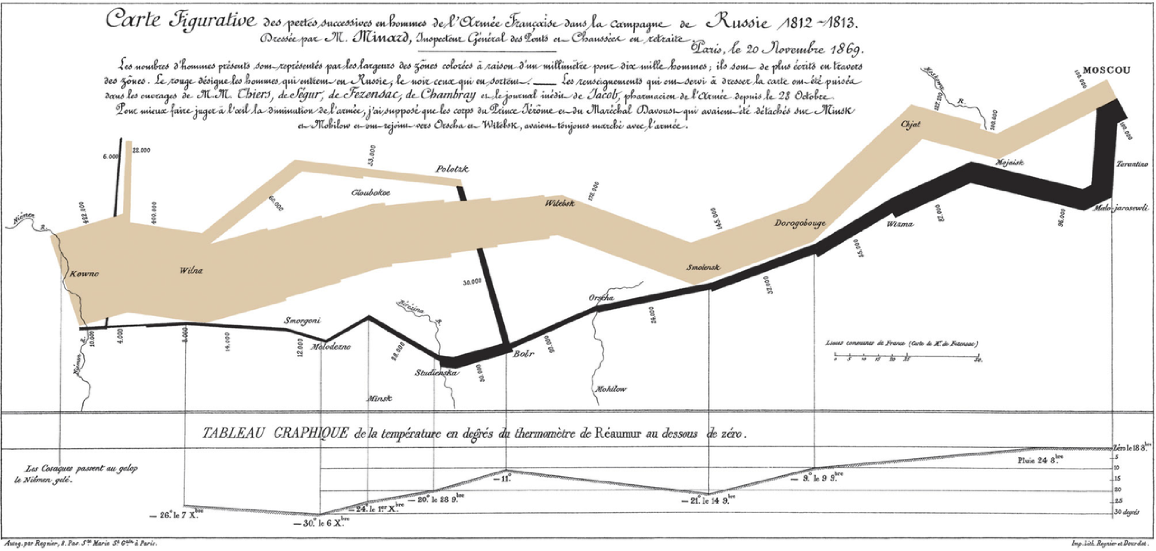
The graph is drawn over a map of eastern Europe. It starts at the Polish-Russian border at the left end. The light brown band represents Napoleon’s army marching towards Moscow, and the black band represents the army returning. At each point of the graph, the width of the band is proportional to the number of soldiers in the army. At the bottom of the graph, Minard includes the temperatures on the return journey.

Notice how narrow the black band becomes as the army heads back. The crossing of the Berezina river was particularly devastating; can you spot it on the graph?

The graph is remarkable for its simplicity and power. In a single graph, Minard shows six variables:

• the number of soldiers
• the direction of the march
• the latitude and longitude of location
• the temperature on the return journey
• the location on specific dates in November and December

Tufte says that Minard’s graph is “probably the best statistical graphic ever drawn.”

Here is a subset of Minard’s data, adapted from The Grammar of Graphics by Leland Wilkinson.

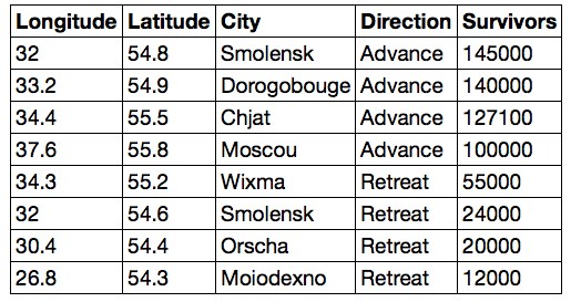
Each row of the column represents the state of the army in a particular location. The columns show the longitude and latitude in degrees, the name of the location, whether the army was advancing or in retreat, and an estimate of the number of men.

In this table the biggest change in the number of men between two consecutive locations is when the retreat begins at Moscow, as is the biggest percentage change.

moscou = 100000
wixma = 55000
wixma - moscou

-45000

(wixma - moscou)/moscou

-0.45

That’s a 45% drop in the number of men in the fighting at Moscow. In other words, almost half of Napoleon’s men who made it into Moscow didn’t get very much farther.

As you can see in the graph, Moiodexno is pretty close to Kowno where the army started out. Fewer than 10% of the men who marched into Smolensk during the advance made it as far as Moiodexno on the way back.

smolensk_A = 145000
moiodexno = 12000
(moiodexno - smolensk_A)/smolensk_A

-0.9172413793103448

Yes, you could do these calculations by just using the numbers without names. But the names make it much easier to read the code and interpret the results.

It is worth noting that bigger absolute changes don’t always correspond to bigger percentage changes.

The absolute loss from Smolensk to Dorogobouge during the advance was 5,000 men, whereas the corresponding loss from Smolensk to Orscha during the retreat was smaller, at 4,000 men.

However, the percent change was much larger between Smolensk and Orscha because the total number of men in Smolensk was much smaller during the retreat.

dorogobouge = 140000
smolensk_R = 24000
orscha = 20000

abs(dorogobouge - smolensk_A)

5000

abs(dorogobouge - smolensk_A)/smolensk_A

0.034482758620689655

abs(orscha - smolensk_R)

4000

abs(orscha - smolensk_R)/smolensk_R

0.16666666666666666