SciPy: high-level scientific computing

Authors: Gaël Varoquaux, Adrien Chauve, Andre Espaze, Emmanuelle Gouillart, Ralf Gommers

Scipy

The scipy package contains various toolboxes dedicated to common issues in scientific computing. Its different submodules correspond to different applications, such as interpolation, integration, optimization, image processing, statistics, special functions, etc.

Note

scipy can be compared to other standard scientific-computing libraries, such as the GSL (GNU Scientific Library for C and C++), or Matlab’s toolboxes. scipy is the core package for scientific routines in Python; it is meant to operate efficiently on numpy arrays, so that NumPy and SciPy work hand in hand.

Before implementing a routine, it is worth checking if the desired data processing is not already implemented in SciPy. As non-professional programmers, scientists often tend to re-invent the wheel, which leads to buggy, non-optimal, difficult-to-share and unmaintainable code. By contrast, SciPy’s routines are optimized and tested, and should therefore be used when possible.

Warning

This tutorial is far from an introduction to numerical computing. As enumerating the different submodules and functions in SciPy would be very boring, we concentrate instead on a few examples to give a general idea of how to use scipy for scientific computing.

scipy is composed of task-specific sub-modules:

scipy.cluster	Vector quantization / Kmeans
scipy.constants	Physical and mathematical constants
scipy.fft	Fourier transform
scipy.integrate	Integration routines
scipy.interpolate	Interpolation
scipy.io	Data input and output
scipy.linalg	Linear algebra routines
scipy.ndimage	n-dimensional image package
scipy.odr	Orthogonal distance regression
scipy.optimize	Optimization
scipy.signal	Signal processing
scipy.sparse	Sparse matrices
scipy.spatial	Spatial data structures and algorithms
scipy.special	Any special mathematical functions
scipy.stats	Statistics

Scipy modules all depend on numpy, but are mostly independent of each other. The standard way of importing NumPy and these SciPy modules is:

import numpy as np
import scipy as sp

We will also be using plotting for this tutorial.

import matplotlib.pyplot as plt

File input/output: scipy.io

scipy.io contains functions for loading and saving data in several common formats including Matlab, IDL, Matrix Market, and Harwell-Boeing.

Matlab files: Loading and saving:

a = np.ones((3, 3))
sp.io.savemat('file.mat', {'a': a})  # savemat expects a dictionary
data = sp.io.loadmat('file.mat')
data['a']

array([[1., 1., 1.],
       [1., 1., 1.],
       [1., 1., 1.]])

Warning — Python / Matlab mismatch

The Matlab file format does not support 1D arrays.

a = np.ones(3)
a

array([1., 1., 1.])

a.shape

(3,)

sp.io.savemat('file.mat', {'a': a})
a2 = sp.io.loadmat('file.mat')['a']
a2

array([[1., 1., 1.]])

a2.shape

(1, 3)

Notice that the original array was a one-dimensional array, whereas the saved and reloaded array is a two-dimensional array with a single row.

For other formats, see the scipy.io documentation.

End of warning

See also

• Load text files: numpy.loadtxt()/numpy.savetxt()

• Clever loading of text/csv files: numpy.genfromtxt()

• Fast and efficient, but NumPy-specific, binary format: numpy.save()/numpy.load()

• Basic input/output of images in Matplotlib: matplotlib.pyplot.imread()/matplotlib.pyplot.imsave()

• More advanced input/output of images: imageio

Special functions: scipy.special

“Special” functions are functions commonly used in science and mathematics that are not considered to be “elementary” functions. Examples include

• the gamma function, scipy.special.gamma(),

• the error function, scipy.special.erf(),

• Bessel functions, such as scipy.special.jv() (Bessel function of the first kind), and

• elliptic functions, such as scipy.special.ellipj() (Jacobi elliptic functions).

Other special functions are combinations of familiar elementary functions, but they offer better accuracy or robustness than their naive implementations would.

Most of these function are computed elementwise and follow standard NumPy broadcasting rules when the input arrays have different shapes. For example, scipy.special.xlog1py() is mathematically equivalent to \(x\log(1 + y)\).

x = np.asarray([1, 2])
y = np.asarray([[3], [4], [5]])
res = sp.special.xlog1py(x, y)
res.shape

(3, 2)

ref = x * np.log(1 + y)
np.allclose(res, ref)

True

However, scipy.special.xlog1py() is numerically favorable for small \(y\), when explicit addition of 1 would lead to loss of precision due to floating point truncation error.

x = 2.5
y = 1e-18
x * np.log(1 + y)

np.float64(0.0)

sp.special.xlog1py(x, y)

np.float64(2.5e-18)

Many special functions also have “logarithmized” variants. For instance, the gamma function \(\Gamma(\cdot)\) is related to the factorial function by \(n! = \Gamma(n + 1)\), but it extends the domain from the positive integers to the complex plane.

x = np.arange(10)
np.allclose(sp.special.gamma(x + 1), sp.special.factorial(x))

True

sp.special.gamma(5) < sp.special.gamma(5.5) < sp.special.gamma(6)

np.True_

The factorial function grows quickly, and so the gamma function overflows for moderate values of the argument. However, sometimes only the logarithm of the gamma function is needed. In such cases, we can compute the logarithm of the gamma function directly using scipy.special.gammaln().

x = [5, 50, 500]
np.log(sp.special.gamma(x))

array([  3.17805383, 144.56574395,          inf])

sp.special.gammaln(x)

array([   3.17805383,  144.56574395, 2605.11585036])

Such functions can often be used when the intermediate components of a calculation would overflow or underflow, but the final result would not. For example, suppose we wish to compute the ratio \(\Gamma(500)/\Gamma(499)\).

a = sp.special.gamma(500)
b = sp.special.gamma(499)
a, b

(np.float64(inf), np.float64(inf))

Both the numerator and denominator overflow, so performing \(a / b\) will not return the result we seek. However, the magnitude of the result should be moderate, so the use of logarithms comes to mind. Combining the identities \(\log(a/b) = \log(a) - \log(b)\) and \(\exp(\log(x)) = x\), we get:

log_a = sp.special.gammaln(500)
log_b = sp.special.gammaln(499)
log_res = log_a - log_b
res = np.exp(log_res)
res

np.float64(499.00000000006696)

Similarly, suppose we wish to compute the difference \(\log(\Gamma(500) - \Gamma(499))\). For this, we use scipy.special.logsumexp(), which computes \(\log(\exp(x) + \exp(y))\) using a numerical trick that avoids overflow.

res = sp.special.logsumexp([log_a, log_b],
                            b=[1, -1])  # weights the terms of the sum
res

np.float64(2605.1138443430073)

For more information about these and many other special functions, see the documentation of scipy.special.

Linear algebra operations: scipy.linalg

scipy.linalg provides a Python interface to efficient, compiled implementations of standard linear algebra operations: the BLAS (Basic Linear Algebra Subroutines) and LAPACK (Linear Algebra PACKage) libraries.

For example, the scipy.linalg.det() function computes the determinant of a square matrix:

arr = np.array([[1, 2],
                [3, 4]])
sp.linalg.det(arr)

np.float64(-2.0)

Mathematically, the solution of a linear system \(Ax = b\) is \(x = A^{-1}b\), but explicit inversion of a matrix is numerically unstable and should be avoided. Instead, use scipy.linalg.solve():

A = np.array([[1, 2],
              [2, 3]])
b = np.array([14, 23])
x = sp.linalg.solve(A, b)
x

array([4., 5.])

np.allclose(A @ x, b)

True

Linear systems with special structure can often be solved more efficiently than more general systems. For example, systems with triangular matrices can be solved using scipy.linalg.solve_triangular():

A_upper = np.triu(A)
A_upper

array([[1, 2],
       [0, 3]])

np.allclose(sp.linalg.solve_triangular(A_upper, b, lower=False),
            sp.linalg.solve(A_upper, b))

True

scipy.linalg also features matrix factorizations/decompositions such as the singular value decomposition.

A = np.array([[1, 2],
              [2, 3]])
U, s, Vh = sp.linalg.svd(A)
s  # singular values

array([4.23606798, 0.23606798])

The original matrix can be recovered by matrix multiplication of the factors:

S = np.diag(s)  # convert to diagonal matrix before matrix multiplication
A2 = U @ S @ Vh
np.allclose(A2, A)

True

A3 = (U * s) @ Vh  # more efficient: use array math broadcasting rules!
np.allclose(A3, A)

True

Many other decompositions (e.g. LU, Cholesky, QR), solvers for structured linear systems (e.g. triangular, circulant), eigenvalue problem algorithms, matrix functions (e.g. matrix exponential), and routines for special matrix creation (e.g. block diagonal, toeplitz) are available in scipy.linalg.

Interpolation: scipy.interpolate

scipy.interpolate is used for fitting a function – an “interpolant” – to experimental or computed data. Once fit, the interpolant can be used to approximate the underlying function at intermediate points; it can also be used to compute the integral, derivative, or inverse of the function.

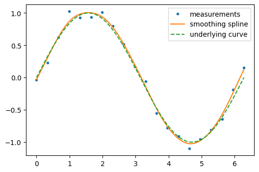
Some kinds of interpolants, known as “smoothing splines”, are designed to generate smooth curves from noisy data. For example, suppose we have the following data:

rng = np.random.default_rng(27446968)

measured_time = np.linspace(0, 2 * np.pi, 20)
function = np.sin(measured_time)
noise = rng.normal(loc=0, scale=0.1, size=20)
measurements = function + noise

scipy.interpolate.make_smoothing_spline() can be used to form a curve similar to the underlying sine function.

smoothing_spline = sp.interpolate.make_smoothing_spline(measured_time, measurements)
interpolation_time = np.linspace(0, 2 * np.pi, 200)
smooth_results = smoothing_spline(interpolation_time)

Show code cell source

Hide code cell source

plt.figure(figsize=(6, 4))
plt.plot(measured_time, measurements, ".", ms=6, label="measurements")
plt.plot(interpolation_time, smooth_results, label="smoothing spline")
plt.plot(interpolation_time, np.sin(interpolation_time), "--", label="underlying curve")
plt.legend();

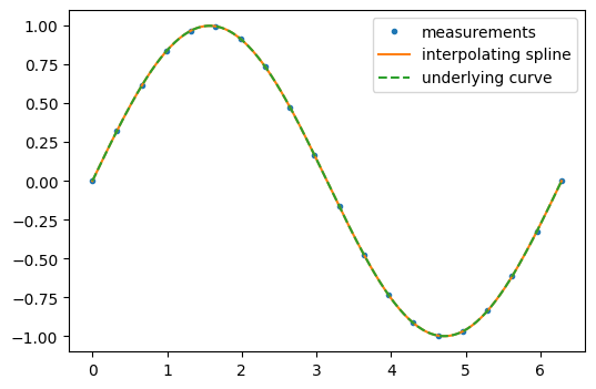
On the other hand, if the data are not noisy, it may be desirable to pass exactly through each point.

interp_spline = sp.interpolate.make_interp_spline(measured_time, function)
interp_results = interp_spline(interpolation_time)

Show code cell source

Hide code cell source

# Plot the data, the interpolant, and the original function
plt.figure(figsize=(6, 4))
plt.plot(measured_time, function, ".", ms=6, label="measurements")
plt.plot(interpolation_time, interp_results, label="interpolating spline")
plt.plot(interpolation_time, np.sin(interpolation_time), "--", label="underlying curve")
plt.legend();

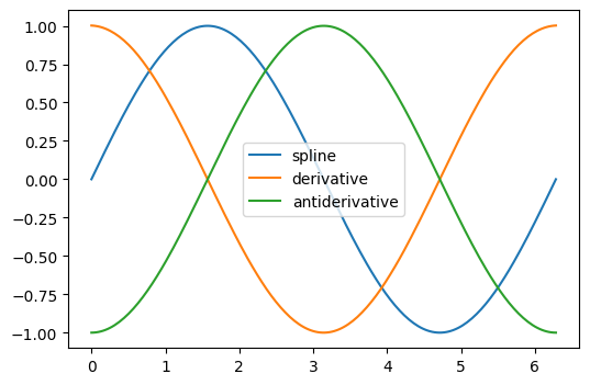
The derivative and antiderivative methods of the result object can be used for differentiation and integration. For the latter, the constant of integration is assumed to be zero, but we can “wrap” the antiderivative to include a nonzero constant of integration.

d_interp_spline = interp_spline.derivative()
d_interp_results = d_interp_spline(interpolation_time)
i_interp_spline = lambda t: interp_spline.antiderivative()(t) - 1
i_interp_results = i_interp_spline(interpolation_time)

Show code cell source

Hide code cell source

# Plot interpolant, its derivative, and its antiderivative
plt.figure(figsize=(6, 4))
t = interpolation_time
plt.plot(t, interp_results, label="spline")
plt.plot(t, d_interp_results, label="derivative")
plt.plot(t, i_interp_results, label="antiderivative")
plt.legend();

For functions that are monotonic on an interval (e.g. \(\sin\) from \(\pi/2\) to \(3\pi/2\)), we can reverse the arguments of make_interp_spline to interpolate the inverse function. Because the first argument is expected to be monotonically increasing, we also reverse the order of elements in the arrays with numpy.flip().

i = (measured_time > np.pi/2) & (measured_time < 3*np.pi/2)
inverse_spline = sp.interpolate.make_interp_spline(np.flip(function[i]),
                                                   np.flip(measured_time[i]))
inverse_spline(0)

array(3.14159265)

See the summary exercise on Maximum wind speed prediction at the Sprogø station for a more advanced spline interpolation example, and read the SciPy interpolation tutorial and the scipy.interpolate documentation for much more information.

Optimization and fit: scipy.optimize

scipy.optimize provides algorithms for root finding, curve fitting, and more general optimization.

Root Finding

scipy.optimize.root_scalar() attempts to find a root of a specified scalar-valued function (i.e., an argument at which the function value is zero). Like many scipy.optimize functions, the function needs an initial guess of the solution, which the algorithm will refine until it converges or recognizes failure. We also provide the derivative to improve the rate of convergence.

def f(x):
    return (x-1)*(x-2)

def df(x):
    return 2*x - 3

x0 = 0  # guess
res = sp.optimize.root_scalar(f, x0=x0, fprime=df)
res

      converged: True
           flag: converged
 function_calls: 12
     iterations: 6
           root: 1.0
         method: newton

Warning

None of the functions in scipy.optimize that accept a guess are guaranteed to converge for all possible guesses! (For example, try x0=1.5 in the example above, where the derivative of the function is exactly zero.) If this occurs, try a different guess, adjust the options (like providing a bracket as shown below), or consider whether SciPy offers a more appropriate method for the problem.

Note that only one the root at 1.0 is found. By inspection, we can tell that there is a second root at 2.0. We can direct the function toward a particular root by changing the guess or by passing a bracket that contains only the root we seek.

res = sp.optimize.root_scalar(f, bracket=(1.5, 10))
res.root

2.0

For multivariate problems, use scipy.optimize.root().

def f(x):
    # intersection of unit circle and line from origin
    return [x[0]**2 + x[1]**2 - 1,
            x[1] - x[0]]

res = sp.optimize.root(f, x0=[0, 0])
np.allclose(f(res.x), 0, atol=1e-10)

True

np.allclose(res.x, np.sqrt(2)/2)

True

Over-constrained problems can be solved in the least-squares sense using scipy.optimize.root() with method='lm' (Levenberg-Marquardt).

def f(x):
    # intersection of unit circle, line from origin, and parabola
    return [x[0]**2 + x[1]**2 - 1,
            x[1] - x[0],
            x[1] - x[0]**2]

res = sp.optimize.root(f, x0=[1, 1], method='lm')
res.success

True

res.x

array([0.76096066, 0.66017736])

See the documentation of scipy.optimize.root_scalar() and scipy.optimize.root() for a variety of other solution algorithms and options.

Curve fitting

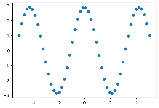
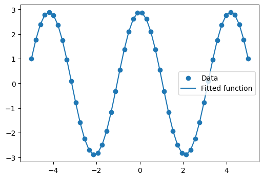
Suppose we have data that is sinusoidal but noisy:

x_data = np.linspace(-5, 5, num=50)  # 50 values between -5 and 5
noise = 0.01 * np.cos(100 * x_data)
a, b = 2.9, 1.5
y_data = a * np.cos(b * x_data) + noise

Show code cell source

Hide code cell source

plt.figure(figsize=(6, 4))
plt.scatter(x_data, y_data);

We can approximate the underlying amplitude, frequency, and phase from the data by least squares curve fitting. To begin, we write a function that accepts the independent variable as the first argument and all parameters to fit as separate arguments:

def f(x, a, b, c):
    return a * np.sin(b * x + c)

We then use scipy.optimize.curve_fit() to find \(a\) and \(b\):

params, _ = sp.optimize.curve_fit(f, x_data, y_data, p0=[2, 1, 3])
params

array([2.900026  , 1.50012043, 1.57079633])

ref = [a, b, np.pi/2]  # what we'd expect
np.allclose(params, ref, rtol=1e-3)

True

We plot the resulting curve on the data:

Show code cell source

Hide code cell source

plt.figure(figsize=(6, 4))
plt.scatter(x_data, y_data, label="Data")
plt.plot(x_data, f(x_data, *params), label="Fitted function")
plt.legend(loc="best");

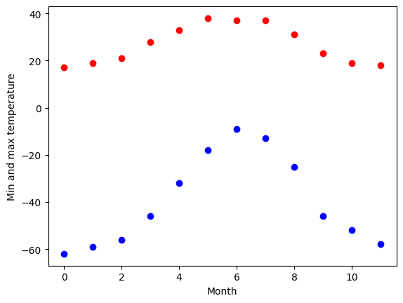
Exercise 39

The temperature extremes in Alaska for each month, starting in January, are given by (in degrees Celsius):

max:  17,  19,  21,  28,  33,  38, 37,  37,  31,  23,  19,  18
min: -62, -59, -56, -46, -32, -18, -9, -13, -25, -46, -52, -58

1. Plot these temperature extremes.

2. Define a function that can describe min and max temperatures. Hint: this function has to have a period of 1 year. Hint: include a time offset.

3. Fit this function to the data with scipy.optimize.curve_fit().

4. Plot the result. Is the fit reasonable? If not, why?

5. Is the time offset for min and max temperatures the same within the fit accuracy?

Solution to Exercise 39

Curve fitting: temperature as a function of month of the year

We have the min and max temperatures in Alaska for each months of the year. We would like to find a function to describe this yearly evolution.

For this, we will fit a periodic function.

# The data
temp_max = np.array([17, 19, 21, 28, 33, 38, 37, 37, 31, 23, 19, 18])
temp_min = np.array([-62, -59, -56, -46, -32, -18, -9, -13, -25, -46, -52, -58])

months = np.arange(12)
plt.plot(months, temp_max, "ro")
plt.plot(months, temp_min, "bo")
plt.xlabel("Month")
plt.ylabel("Min and max temperature");

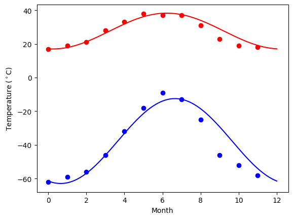
Fitting it to a periodic function:

def yearly_temps(times, avg, ampl, time_offset):
    return avg + ampl * np.cos((times + time_offset) * 2 * np.pi / times.max())

res_max, cov_max = sp.optimize.curve_fit(yearly_temps, months, temp_max, [20, 10, 0])
res_min, cov_min = sp.optimize.curve_fit(yearly_temps, months, temp_min, [-40, 20, 0])

Plotting the fit

days = np.linspace(0, 12, num=365)
plt.figure()
plt.plot(months, temp_max, "ro")
plt.plot(days, yearly_temps(days, *res_max), "r-")
plt.plot(months, temp_min, "bo")
plt.plot(days, yearly_temps(days, *res_min), "b-")
plt.xlabel("Month")
plt.ylabel(r"Temperature ($^\circ$C)");

Optimization

Suppose we wish to minimize the scalar-valued function of a single variable \(f(x) = x^2 + 10 \sin(x)\):

def f(x):
    return x**2 + 10 * np.sin(x)

x = np.arange(-5, 5, 0.1)
plt.plot(x, f(x))

[<matplotlib.lines.Line2D at 0x10ac38e90>]

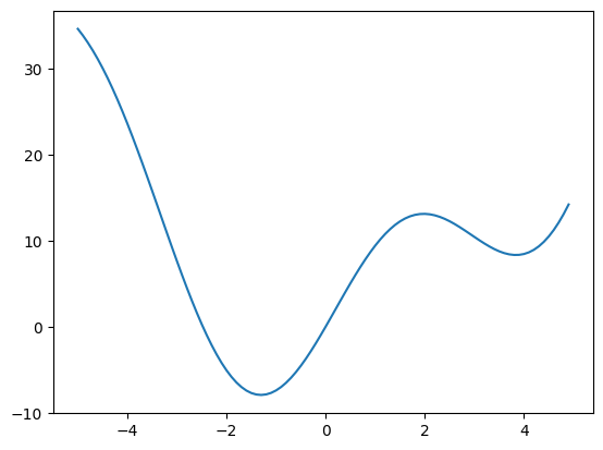
We can see that the function has a local minimizer near \(x = 3.8\) and a global minimizer near \(x = -1.3\), but the precise values cannot be determined from the plot.

The most appropriate function for this purpose is scipy.optimize.minimize_scalar(). Since we know the approximate locations of the minima, we will provide bounds that restrict the search to the vicinity of the global minimum.

res = sp.optimize.minimize_scalar(f, bounds=(-2, -1))
res

 message: Solution found.
 success: True
  status: 0
     fun: -7.9458233756095895
       x: -1.3064409970312618
     nit: 8
    nfev: 8

res.fun == f(res.x)

np.True_

If we did not already know the approximate location of the global minimum, we could use one of SciPy’s global minimizers, such as scipy.optimize.differential_evolution(). We are required to pass bounds, but they do not need to be tight.

bounds=[(-5, 5)]  # list of lower, upper bound for each variable
res = sp.optimize.differential_evolution(f, bounds=bounds)
res

             message: Optimization terminated successfully.
             success: True
                 fun: -7.945823375615284
                   x: [-1.306e+00]
                 nit: 6
                nfev: 113
          population: [[-1.303e+00]
                       [-1.231e+00]
                       ...
                       [-1.289e+00]
                       [-1.321e+00]]
 population_energies: [-7.946e+00 -7.913e+00 ... -7.944e+00 -7.945e+00]
                 jac: [ 8.882e-08]

For multivariate optimization, a good choice for many problems is scipy.optimize.minimize(). Suppose we wish to find the minimum of a quadratic function of two variables, \(f(x_0, x_1) = (x_0-1)^2 + (x_1-2)^2\).

def f(x):
    return (x[0] - 1)**2 + (x[1] - 2)**2

Like scipy.optimize.root(), scipy.optimize.minimize() requires a guess x0. (Note that this is the initial value of both variables rather than the value of the variable we happened to label \(x_0\).)

res = sp.optimize.minimize(f, x0=[0, 0])
res

  message: Optimization terminated successfully.
  success: True
   status: 0
      fun: 1.705780445775116e-16
        x: [ 1.000e+00  2.000e+00]
      nit: 2
      jac: [ 3.219e-09 -8.462e-09]
 hess_inv: [[ 9.000e-01 -2.000e-01]
            [-2.000e-01  6.000e-01]]
     nfev: 9
     njev: 3

Maximization?

Is scipy.optimize.minimize() restricted to the solution of minimization problems? Nope! To solve a maximization problem, simply minimize the negative of the original objective function.

This barely scratches the surface of SciPy’s optimization features, which include mixed integer linear programming, constrained nonlinear programming, and the solution of assignment problems. For much more information, see the documentation of scipy.optimize and the advanced chapter Mathematical optimization: finding minima of functions.

Exercise 40

This is an exercise on 2-D minimization.

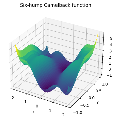
The six-hump camelback function

\(f(x, y) = (4 - 2.1x^2 + \frac{x^4}{3})x^2 + xy + (4y^2 - 4)y^2\)

has multiple local minima. Find a global minimum (there is more than one, each with the same value of the objective function) and at least one other local minimum.

Hints:

• Variables can be restricted to \(-2 < x < 2\) and \(-1 < y < 1\).

• numpy.meshgrid() and matplotlib.pyplot.imshow() can help with visualization.

• Try minimizing with scipy.optimize.minimize() with an initial guess of \((x, y) = (0, 0)\). Does it find the global minimum, or converge to a local minimum? What about other initial guesses?

• Try minimizing with scipy.optimize.differential_evolution().

Solution to Exercise 40

Optimization of a two-parameter function:

# Define the function that we are interested in
def sixhump(x):
    return (
        (4 - 2.1 * x[0] ** 2 + x[0] ** 4 / 3) * x[0] ** 2
        + x[0] * x[1]
        + (-4 + 4 * x[1] ** 2) * x[1] ** 2
    )

# Make a grid to evaluate the function (for plotting)
xlim = [-2, 2]
ylim = [-1, 1]
x = np.linspace(*xlim)  # type: ignore[call-overload]
y = np.linspace(*ylim)  # type: ignore[call-overload]
xg, yg = np.meshgrid(x, y)

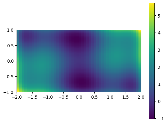
A 2D image plot of the function:

# Simple visualization in 2D
plt.figure()
plt.imshow(sixhump([xg, yg]), extent=xlim + ylim, origin="lower")  # type: ignore[arg-type]
plt.colorbar();

A 3D surface plot of the function:

from mpl_toolkits.mplot3d import Axes3D

fig = plt.figure()
ax: Axes3D = fig.add_subplot(111, projection="3d")
surf = ax.plot_surface(
    xg,
    yg,
    sixhump([xg, yg]),
    rstride=1,
    cstride=1,
    cmap="viridis",
    linewidth=0,
    antialiased=False,
)

ax.set_xlabel("x")
ax.set_ylabel("y")
ax.set_zlabel("f(x, y)")
ax.set_title("Six-hump Camelback function");

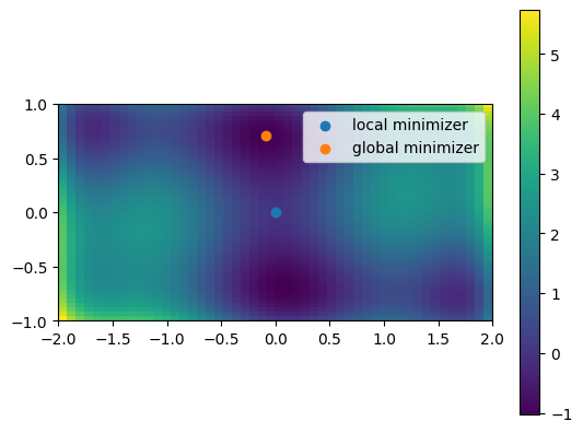
Find minima:

# local minimization
res_local = sp.optimize.minimize(sixhump, x0=[0, 0])
# global minimization
res_global = sp.optimize.differential_evolution(sixhump, bounds=[xlim, ylim])

Show code cell source

Hide code cell source

plt.figure()
# Show the function in 2D
plt.imshow(sixhump([xg, yg]), extent=xlim + ylim, origin="lower")  # type: ignore[arg-type]
plt.colorbar()
# Mark the minima
plt.scatter(res_local.x[0], res_local.x[1], label="local minimizer")
plt.scatter(res_global.x[0], res_global.x[1], label="global minimizer")
plt.legend();

See the summary exercise on Non linear least squares curve fitting: application to point extraction in topographical lidar data for another, more advanced example.

Statistics and random numbers: scipy.stats

scipy.stats contains fundamental tools for statistics in Python.

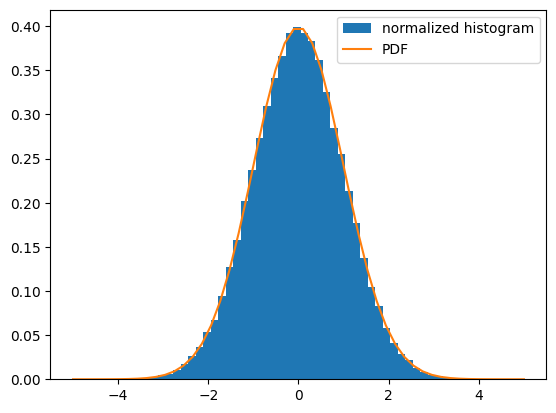
Statistical Distributions

Consider a random variable distributed according to the standard normal. We draw a sample consisting of 100000 observations from the random variable. The normalized histogram of the sample is an estimator of the random variable’s probability density function (PDF):

dist = sp.stats.norm(loc=0, scale=1)  # standard normal distribution
sample = dist.rvs(size=100000)  # "random variate sample"
plt.hist(sample, bins=50, density=True, label='normalized histogram')
x = np.linspace(-5, 5)
plt.plot(x, dist.pdf(x), label='PDF')
plt.legend()

<matplotlib.legend.Legend at 0x10bc7a180>

Distribution objects and frozen distributions

Each of the 100+ scipy.stats distribution families is represented by an object with a __call__ method. Here, we call the scipy.stats.norm object to specify its location and scale, and it returns a frozen distribution: a particular element of a distribution family with all parameters fixed. The frozen distribution object has methods to compute essential functions of the particular distribution.

Suppose we knew that the sample had been drawn from a distribution belonging to the family of normal distributions, but we did not know the particular distribution’s location (mean) and scale (standard deviation). We perform maximum likelihood estimation of the unknown parameters using the distribution family’s fit method:

loc, scale = sp.stats.norm.fit(sample)
loc

np.float64(0.004670820735986828)

scale

np.float64(1.0004755498549254)

Since we know the true parameters of the distribution from which the sample was drawn, we are not surprised that these estimates are similar.

Exercise 41

Generate 1000 random variates from a gamma distribution with a shape parameter of 1. Hint: the shape parameter is passed as the first argument when freezing the distribution. Plot the histogram of the sample, and overlay the distribution’s PDF. Estimate the shape parameter from the sample using the fit method.

Extra: the distributions have many useful methods. Explore them using tab completion. Plot the cumulative density function of the distribution, and compute the variance.

Sample Statistics and Hypothesis Tests

The sample mean is an estimator of the mean of the distribution from which the sample was drawn:

np.mean(sample)

np.float64(0.004670820735986828)

NumPy includes some of the most fundamental sample statistics (e.g. numpy.mean(), numpy.var(), numpy.percentile()); scipy.stats includes many more. For instance, the geometric mean is a common measure of central tendency for data that tends to be distributed over many orders of magnitude.

sp.stats.gmean(2**sample)

np.float64(1.0032428128020978)

SciPy also includes a variety of hypothesis tests that produce a sample statistic and a p-value. For instance, suppose we wish to test the null hypothesis that sample was drawn from a normal distribution:

res = sp.stats.normaltest(sample)
res.statistic

np.float64(1.0119533941689594)

res.pvalue

np.float64(0.6029164210505692)

Here, statistic is a sample statistic that tends to be high for samples that are drawn from non-normal distributions. pvalue is the probability of observing such a high value of the statistic for a sample that has been drawn from a normal distribution. If the p-value is unusually small, this may be taken as evidence that sample was not drawn from the normal distribution. Our statistic and p-value are moderate, so the test is inconclusive.

There are many other features of scipy.stats, including circular statistics, quasi-Monte Carlo methods, and resampling methods. For much more information, see the documentation of scipy.stats and the advanced chapter statistics.

Numerical integration: scipy.integrate

Quadrature

Suppose we wish to compute the definite integral \(\int_0^{\pi / 2} \sin(t) dt\) numerically. scipy.integrate.quad() chooses one of several adaptive techniques depending on the parameters, and is therefore the recommended first choice for integration of function of a single variable:

integral, error_estimate = sp.integrate.quad(np.sin, 0, np.pi / 2)
np.allclose(integral, 1)  # numerical result ~ analytical result

True

abs(integral - 1) < error_estimate  #  actual error < estimated error

True

Other functions for numerical quadrature, including integration of multivariate functions and approximating integrals from samples, are available in scipy.integrate.

Initial Value Problems

scipy.integrate also features routines for integrating Ordinary Differential Equations (ODE). For example, scipy.integrate.solve_ivp() integrates ODEs of the form:

\[ \frac{dy}{dt} = f(t, y(t)) \]

from an initial time \(t_0\) and initial state \(y(t=t_0)=t_0\) to a final time \(t_f\) or until an event occurs (e.g. a specified state is reached).

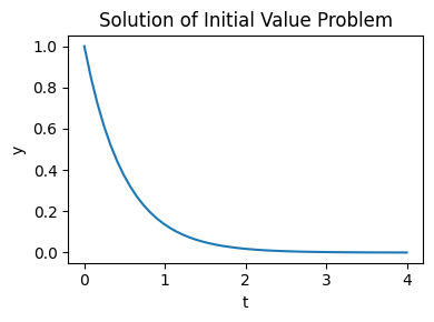
As an introduction, consider the initial value problem given by \(\frac{dy}{dt} = -2 y\) and the initial condition \(y(t=0) = 1\) on the interval \(t = 0 \dots 4\). We begin by defining a callable that computes \(f(t, y(t))\) given the current time and state.

def f(t, y):
    return -2 * y

Then, to compute y as a function of time:

t_span = (0, 4)  # time interval
t_eval = np.linspace(*t_span)  # times at which to evaluate `y`
y0 = [1,]  # initial state
res = sp.integrate.solve_ivp(f, t_span=t_span, y0=y0, t_eval=t_eval)

and plot the result:

plt.figure(figsize=(4, 3))
plt.plot(res.t, res.y[0])
plt.xlabel('t')
plt.ylabel('y')
plt.title('Solution of Initial Value Problem')
plt.tight_layout();

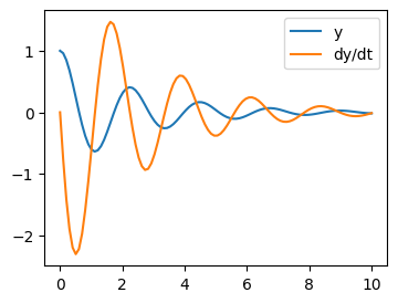
Let us integrate a more complex ODE: a damped spring-mass oscillator. The position of a mass attached to a spring obeys the 2nd order ODE \(\ddot{y} + 2 \zeta \omega_0 \dot{y} + \omega_0^2 y = 0\) with natural frequency \(\omega_0 = \sqrt{k/m}\), damping ratio \(\zeta = c/(2 m \omega_0)\), spring constant \(k\), mass \(m\), and damping coefficient \(c\).

Before using scipy.integrate.solve_ivp(), the 2nd order ODE needs to be transformed into a system of first-order ODEs. Note that

\[ \frac{dy}{dt} = \dot{y} \frac{d\dot{y}}{dt} = \ddot{y} = -(2 \zeta \omega_0 \dot{y} + \omega_0^2 y) \]

If we define \(z = [z_0, z_1]\) where \(z_0 = y\) and \(z_1 = \dot{y}\), then the first order equation:

\[\begin{split} \frac{dz}{dt} = \begin{bmatrix} \frac{dz_0}{dt} \\ \frac{dz_1}{dt} \end{bmatrix} = \begin{bmatrix} z_1 \\ -(2 \zeta \omega_0 z_1 + \omega_0^2 z_0) \end{bmatrix} \end{split}\]

is equivalent to the original second order equation.

We set:

m = 0.5  # kg
k = 4  # N/m
c = 0.4  # N s/m
zeta = c / (2 * m * np.sqrt(k/m))
omega = np.sqrt(k / m)

and define the function that computes \(\dot{z} = f(t, z(t))\):

def f(t, z, zeta, omega):
    return (z[1], -2.0 * zeta * omega * z[1] - omega**2 * z[0])

Integration of the system follows:

t_span = (0, 10)
t_eval = np.linspace(*t_span, 100)
z0 = [1, 0]
res = sp.integrate.solve_ivp(f, t_span, z0, t_eval=t_eval,
                             args=(zeta, omega), method='LSODA')

Show code cell source

Hide code cell source

plt.figure(figsize=(4, 3))
plt.plot(res.t, res.y[0], label="y")
plt.plot(res.t, res.y[1], label="dy/dt")
plt.legend(loc="best");

Note

With the option method='LSODA', scipy.integrate.solve_ivp() uses the LSODA (Livermore Solver for Ordinary Differential equations with Automatic method switching for stiff and non-stiff problems). See the [ODEPACK Fortran library] for more details.

See also

Partial Differental Equations

There is no Partial Differential Equations (PDE) solver in SciPy. Some Python packages for solving PDE’s are available, such as [fipy] or [SfePy].

Fast Fourier transforms: scipy.fft

The scipy.fft module computes fast Fourier transforms (FFTs) and offers utilities to handle them. Some important functions are:

• scipy.fft.fft() to compute the FFT

• scipy.fft.fftfreq() to generate the sampling frequencies

• scipy.fft.ifft() to compute the inverse FFT, from frequency space to signal space

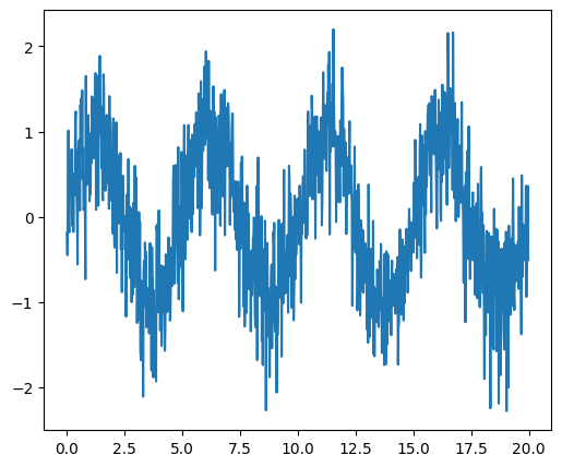
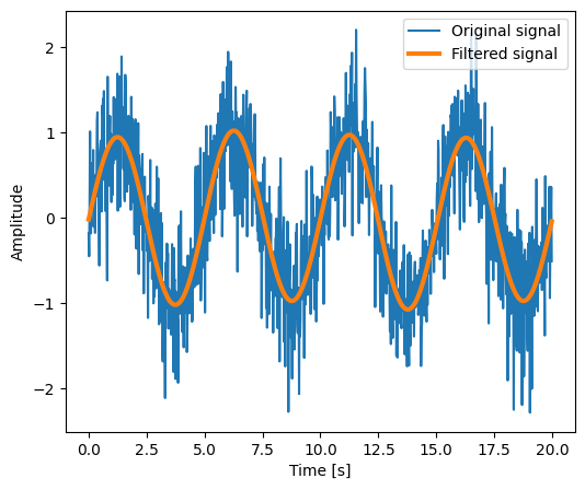
As an illustration, a example (noisy) input signal (sig), and its FFT:

# Time.
dt = 0.02  # Time step.
t = np.arange(0, 20, dt)  # Time vector.
# An example noisy signal over time.
sig = np.sin(2 * np.pi / 5.0 * t) + 0.5 * rng.normal(size=t.size)
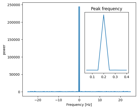
# FFT of signal.
sig_fft = sp.fft.fft(sig)
# Corresponding frequencies.
freqs = sp.fft.fftfreq(sig.size, d=dt)

Signal	FFT

The peak signal frequency can be found with freqs[power.argmax()].

The code of this example and the figures above can be found in the Scipy FFT example.

Setting the Fourier component above this frequency to zero and inverting the FFT with scipy.fft.ifft(), gives a filtered signal (see the example for detail).

numpy.fft

NumPy also has an implementation of FFT (numpy.fft). However, the SciPy one should be preferred, as it uses more efficient underlying implementations.

Fully worked examples:

Crude periodicity finding	Image blur with FFT

Exercise 42

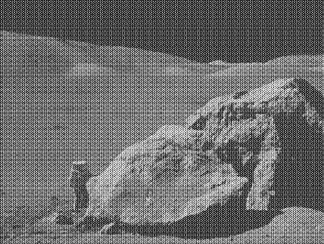
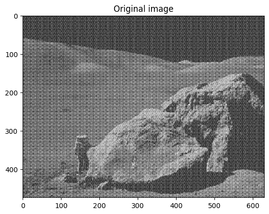
1. Examine the provided image moonlanding.png, which is heavily contaminated with periodic noise. In this exercise, we aim to clean up the noise using the Fast Fourier Transform.

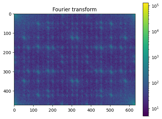
2. Load the image using matplotlib.pyplot.imread().

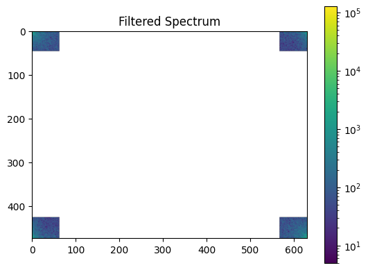
3. Find and use the 2-D FFT function in scipy.fft, and plot the spectrum (Fourier transform of) the image. Do you have any trouble visualising the spectrum? If so, why?

4. The spectrum consists of high and low frequency components. The noise is contained in the high-frequency part of the spectrum, so set some of those components to zero (use array slicing).

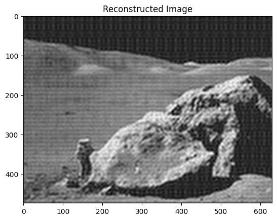
5. Apply the inverse Fourier transform to see the resulting image.

Solution to Exercise 42

Implementing image denoising with FFT.

Denoise an image (data/moonlanding.png) by implementing a blur with an FFT.

Implements, via FFT, the following convolution:

\[\begin{split} \begin{align} f_1(t) = \int dt'\, K(t-t') f_0(t') \\ \tilde{f}_1(\omega) = \tilde{K}(\omega) \tilde{f}_0(\omega) \end{align} \end{split}\]

# Read and plot the image
im = plt.imread("data/moonlanding.png").astype(float)

plt.figure()
plt.imshow(im, "gray")
plt.title("Original image");

# Compute the 2d FFT of the input image
im_fft = sp.fft.fft2(im)

# Show the results
from matplotlib.colors import LogNorm

def plot_spectrum(im_fft):
    # A logarithmic colormap
    plt.imshow(np.abs(im_fft), norm=LogNorm(vmin=5))
    plt.colorbar()

plt.figure()
plot_spectrum(im_fft)
plt.title("Fourier transform");

Filter in FFT:

In the lines following, we’ll make a copy of the original spectrum and truncate coefficients.

# Define the fraction of coefficients (in each direction) we keep
keep_fraction = 0.1

# Call ff a copy of the original transform. NumPy arrays have a copy
# method for this purpose.
im_fft2 = im_fft.copy()

# Set r and c to be the number of rows and columns of the array.
r, c = im_fft2.shape

# Set to zero all rows with indices between r*keep_fraction and
# r*(1-keep_fraction):
im_fft2[int(r * keep_fraction) : int(r * (1 - keep_fraction))] = 0

# Similarly with the columns:
im_fft2[:, int(c * keep_fraction) : int(c * (1 - keep_fraction))] = 0

plt.figure()
plot_spectrum(im_fft2)
plt.title("Filtered Spectrum");

Reconstruct the final image

# Reconstruct the denoised image from the filtered spectrum, keep only the
# real part for display.
im_new = sp.fft.ifft2(im_fft2).real

plt.figure()
plt.imshow(im_new, "gray")
plt.title("Reconstructed Image");

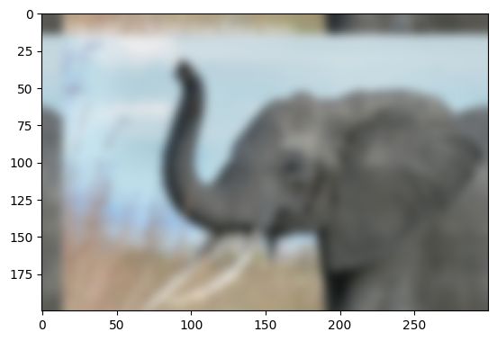
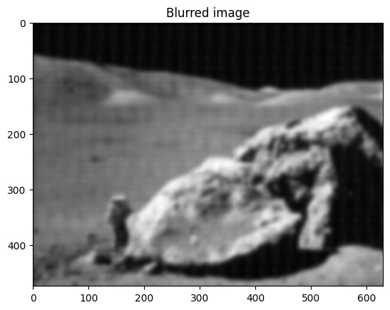
Easier and better: scipy.ndimage.gaussian_filter()

Implementing filtering directly with FFTs is tricky and time consuming. We can use the Gaussian filter from scipy.ndimage

im_blur = sp.ndimage.gaussian_filter(im, 4)

plt.figure()
plt.imshow(im_blur, "gray")
plt.title("Blurred image");

Signal processing: scipy.signal

Note

scipy.signal is for typical signal processing: 1D, regularly-sampled signals.

Resampling scipy.signal.resample(): resample a signal to n points using FFT.

t = np.linspace(0, 5, 100)
x = np.sin(t)

x_resampled = sp.signal.resample(x, 25)

Show code cell source

Hide code cell source

# Plot
plt.figure(figsize=(5, 4))
plt.plot(t, x, label="Original signal")
plt.plot(t[::4], x_resampled, "ko", label="Resampled signal")
plt.legend(loc="best");

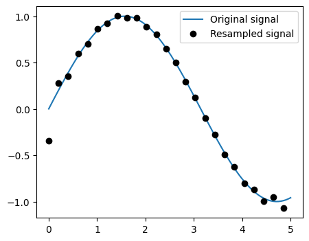
Note

Notice how on the side of the window the resampling is less accurate and has a rippling effect.

This resampling is different from the interpolation provided by scipy.interpolate as it only applies to regularly sampled data.

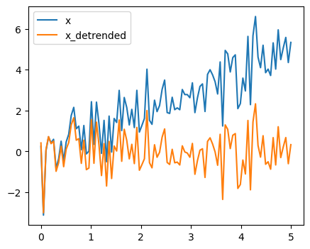
Detrending scipy.signal.detrend(): remove linear trend from signal:

t = np.linspace(0, 5, 100)
rng = np.random.default_rng()
x = t + rng.normal(size=100)

x_detrended = sp.signal.detrend(x)

Show code cell source

Hide code cell source

# Plot
plt.figure(figsize=(5, 4))
plt.plot(t, x, label="x")
plt.plot(t, x_detrended, label="x_detrended")
plt.legend(loc="best");

Filtering:

For non-linear filtering, scipy.signal has filtering (median filter scipy.signal.medfilt(), Wiener scipy.signal.wiener()), but we will discuss this in the image section.

Note

scipy.signal also has a full-blown set of tools for the design of linear filter (finite and infinite response filters), but this is out of the scope of this tutorial.

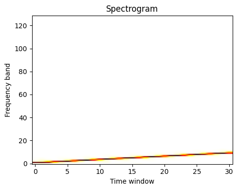
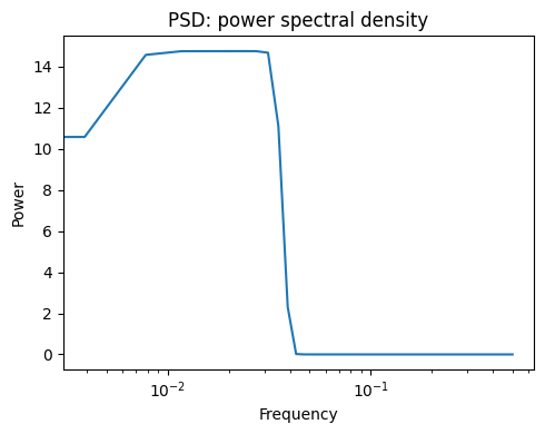
Spectral analysis:

scipy.signal.spectrogram() computes a spectrogram — frequency spectra over consecutive time windows — while scipy.signal.welch() computes a power spectrum density (PSD).

Signal	Spectrogram	Power Spectral Density

See the Spectrogram example.

Image manipulation: scipy.ndimage

See Scipy image processing

Summary exercises on scientific computing

The summary exercises use mainly NumPy, SciPy and Matplotlib. They provide some real-life examples of scientific computing with Python. Now that the basics of working with NumPy and SciPy have been introduced, the interested user is invited to try these exercises.

• Statistical interpolotion

• Non-linear fitting

• Image processing

See also

References to go further

• Some chapters of the advanced and the packages and applications parts of the SciPy lectures.

• The SciPy cookbook

Other useful links

• fipy

• odepack fortran library

• sfepy