Geometrical transformations on images

scipy.ndimage provides manipulation of n-dimensional arrays as images.

import numpy as np
import matplotlib.pyplot as plt

Changing orientation, resolution, ..

import scipy as sp

# Load an image
face = sp.datasets.face(gray=True)

# Shift, rotate and zoom it
shifted_face = sp.ndimage.shift(face, (50, 50))
shifted_face2 = sp.ndimage.shift(face, (50, 50), mode='nearest')
rotated_face = sp.ndimage.rotate(face, 30)
cropped_face = face[50:-50, 50:-50]
zoomed_face = sp.ndimage.zoom(face, 2)
zoomed_face.shape

(1536, 2048)

Show code cell source

Hide code cell source

plt.figure(figsize=(15, 3))
fig, axes = plt.subplots(1, 5)
for i, arr in enumerate([shifted_face,
                         shifted_face2,
                         rotated_face,
                         cropped_face,
                         zoomed_face]):
    axes[i].imshow(arr, cmap="gray")
    axes[i].axis("off")

plt.subplots_adjust(wspace=0.05, left=0.01, bottom=0.01, right=0.99, top=0.99);

<Figure size 1500x300 with 0 Axes>

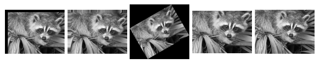
Image filtering

Generate a noisy face:

face = sp.datasets.face(gray=True)
face = face[:512, -512:]  # crop out square on right
noisy_face = np.copy(face).astype(float)
rng = np.random.default_rng()
noisy_face += face.std() * 0.5 * rng.standard_normal(face.shape)

Apply a variety of filters on it:

blurred_face = sp.ndimage.gaussian_filter(noisy_face, sigma=3)
median_face = sp.ndimage.median_filter(noisy_face, size=5)
wiener_face = sp.signal.wiener(noisy_face, (5, 5))

Show code cell source

Hide code cell source

plt.figure(figsize=(12, 3.5))
fig, axes = plt.subplots(1, 4)
for i, (arr, name) in enumerate([[noisy_face, 'noisy'],
                                 [blurred_face, 'Gaussian filter'],
                                 [median_face, 'median filter'],
                                 [wiener_face, 'Wiener filter']]):
    axes[i].imshow(arr, cmap="gray")
    axes[i].set_title(name)
    axes[i].axis("off")

plt.subplots_adjust(wspace=0.05, left=0.01, bottom=0.01, right=0.99, top=0.99)

<Figure size 1200x350 with 0 Axes>

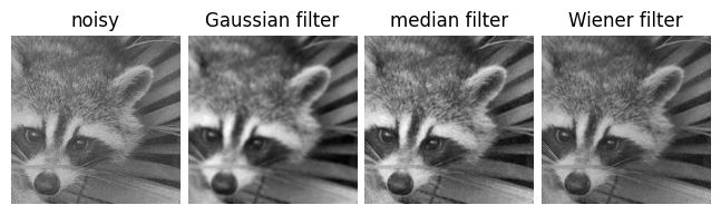
Other filters in scipy.ndimage.filters and scipy.signal can be applied to images.

Compare histograms for the different filtered images.

Mathematical morphology

Note

Mathematical morphology stems from set theory. It characterizes and transforms geometrical structures. Binary (black and white) images, in particular, can be transformed using this theory: the sets to be transformed are the sets of neighboring non-zero-valued pixels. The theory was also extended to gray-valued images.

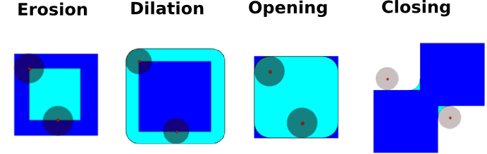
Mathematical-morphology operations use a structuring element in order to modify geometrical structures.

Let us first generate a structuring element:

el = sp.ndimage.generate_binary_structure(2, 1)
el

array([[False,  True, False],
       [ True,  True,  True],
       [False,  True, False]])

el.astype(int)

array([[0, 1, 0],
       [1, 1, 1],
       [0, 1, 0]])

• Erosion scipy.ndimage.binary_erosion()

a = np.zeros((7, 7), dtype=int)
a[1:6, 2:5] = 1
a

array([[0, 0, 0, 0, 0, 0, 0],
       [0, 0, 1, 1, 1, 0, 0],
       [0, 0, 1, 1, 1, 0, 0],
       [0, 0, 1, 1, 1, 0, 0],
       [0, 0, 1, 1, 1, 0, 0],
       [0, 0, 1, 1, 1, 0, 0],
       [0, 0, 0, 0, 0, 0, 0]])

sp.ndimage.binary_erosion(a).astype(a.dtype)

array([[0, 0, 0, 0, 0, 0, 0],
       [0, 0, 0, 0, 0, 0, 0],
       [0, 0, 0, 1, 0, 0, 0],
       [0, 0, 0, 1, 0, 0, 0],
       [0, 0, 0, 1, 0, 0, 0],
       [0, 0, 0, 0, 0, 0, 0],
       [0, 0, 0, 0, 0, 0, 0]])

# Erosion removes objects smaller than the structure
sp.ndimage.binary_erosion(a, structure=np.ones((5,5))).astype(a.dtype)

array([[0, 0, 0, 0, 0, 0, 0],
       [0, 0, 0, 0, 0, 0, 0],
       [0, 0, 0, 0, 0, 0, 0],
       [0, 0, 0, 0, 0, 0, 0],
       [0, 0, 0, 0, 0, 0, 0],
       [0, 0, 0, 0, 0, 0, 0],
       [0, 0, 0, 0, 0, 0, 0]])

• Dilation scipy.ndimage.binary_dilation()

a = np.zeros((5, 5))
a[2, 2] = 1
a

array([[0., 0., 0., 0., 0.],
       [0., 0., 0., 0., 0.],
       [0., 0., 1., 0., 0.],
       [0., 0., 0., 0., 0.],
       [0., 0., 0., 0., 0.]])

sp.ndimage.binary_dilation(a).astype(a.dtype)

array([[0., 0., 0., 0., 0.],
       [0., 0., 1., 0., 0.],
       [0., 1., 1., 1., 0.],
       [0., 0., 1., 0., 0.],
       [0., 0., 0., 0., 0.]])

• Opening scipy.ndimage.binary_opening()

a = np.zeros((5, 5), dtype=int)
a[1:4, 1:4] = 1
a[4, 4] = 1
a

array([[0, 0, 0, 0, 0],
       [0, 1, 1, 1, 0],
       [0, 1, 1, 1, 0],
       [0, 1, 1, 1, 0],
       [0, 0, 0, 0, 1]])

# Opening removes small objects
sp.ndimage.binary_opening(a, structure=np.ones((3, 3))).astype(int)

array([[0, 0, 0, 0, 0],
       [0, 1, 1, 1, 0],
       [0, 1, 1, 1, 0],
       [0, 1, 1, 1, 0],
       [0, 0, 0, 0, 0]])

# Opening can also smooth corners
sp.ndimage.binary_opening(a).astype(int)

array([[0, 0, 0, 0, 0],
       [0, 0, 1, 0, 0],
       [0, 1, 1, 1, 0],
       [0, 0, 1, 0, 0],
       [0, 0, 0, 0, 0]])

• Closing: scipy.ndimage.binary_closing()

Check that opening amounts to eroding, then dilating.

An opening operation removes small structures, while a closing operation fills small holes. Such operations can therefore be used to “clean” an image.

a = np.zeros((50, 50))
a[10:-10, 10:-10] = 1
rng = np.random.default_rng()
a += 0.25 * rng.standard_normal(a.shape)
mask = a>=0.5
opened_mask = sp.ndimage.binary_opening(mask)
closed_mask = sp.ndimage.binary_closing(opened_mask)

Show code cell source

Hide code cell source

plt.figure(figsize=(12, 3.5))
for i, (arr, name) in enumerate([[a, 'a'],
                                 [mask, 'mask'],
                                 [opened_mask, 'opened_mask'],
                                 [closed_mask, 'closed_mask']]):
    axes[i].imshow(shifted_face, cmap="gray")
    axes[i].set_title(name)
    axes[i].axis("off")

plt.subplots_adjust(wspace=0.05, left=0.01, bottom=0.01, right=0.99, top=0.99)

<Figure size 1200x350 with 0 Axes>

Check that the area of the reconstructed square is smaller than the area of the initial square. (The opposite would occur if the closing step was performed before the opening).

For gray-valued images, eroding (resp. dilating) amounts to replacing a pixel by the minimal (resp. maximal) value among pixels covered by the structuring element centered on the pixel of interest.

a = np.zeros((7, 7), dtype=int)
a[1:6, 1:6] = 3
a[4, 4] = 2; a[2, 3] = 1
a

array([[0, 0, 0, 0, 0, 0, 0],
       [0, 3, 3, 3, 3, 3, 0],
       [0, 3, 3, 1, 3, 3, 0],
       [0, 3, 3, 3, 3, 3, 0],
       [0, 3, 3, 3, 2, 3, 0],
       [0, 3, 3, 3, 3, 3, 0],
       [0, 0, 0, 0, 0, 0, 0]])

sp.ndimage.grey_erosion(a, size=(3, 3))

array([[0, 0, 0, 0, 0, 0, 0],
       [0, 0, 0, 0, 0, 0, 0],
       [0, 0, 1, 1, 1, 0, 0],
       [0, 0, 1, 1, 1, 0, 0],
       [0, 0, 3, 2, 2, 0, 0],
       [0, 0, 0, 0, 0, 0, 0],
       [0, 0, 0, 0, 0, 0, 0]])

Connected components and measurements on images

Let us first generate a nice synthetic binary image.

x, y = np.indices((100, 100))
sig = np.sin(2*np.pi*x/50.) * np.sin(2*np.pi*y/50.) * (1+x*y/50.**2)**2
mask = sig > 1

Show code cell source

Hide code cell source

plt.figure(figsize=(7, 3.5))
fig, axes = plt.subplots(1, 2)
axes[0].imshow(sig)
axes[0].axis("off")
axes[0].set_title("sig")
axes[1].imshow(mask, cmap="gray")
axes[1].axis("off")
axes[1].set_title("mask")
plt.subplots_adjust(wspace=0.05, left=0.01, bottom=0.01, right=0.99, top=0.9);

<Figure size 700x350 with 0 Axes>

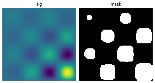
scipy.ndimage.label() assigns a different label to each connected component:

labels, nb = sp.ndimage.label(mask)
nb

8

Show code cell source

Hide code cell source

plt.figure(figsize=(3.5, 3.5))
plt.imshow(labels)
plt.title("label")
plt.axis("off")

plt.subplots_adjust(wspace=0.05, left=0.01, bottom=0.01, right=0.99, top=0.9)

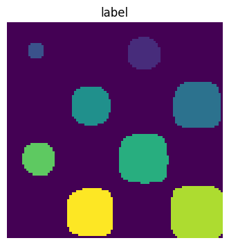
Now compute measurements on each connected component:

areas = sp.ndimage.sum(mask, labels, range(1, labels.max()+1))
areas   # The number of pixels in each connected component

array([190.,  45., 424., 278., 459., 190., 549., 424.])

maxima = sp.ndimage.maximum(sig, labels, range(1, labels.max()+1))
maxima  # The maximum signal in each connected component

array([ 1.80238238,  1.13527605,  5.51954079,  2.49611818,  6.71673619,
        1.80238238, 16.76547217,  5.51954079])

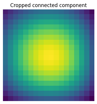
Extract the 4th connected component, and crop the array around it:

sl_3 = sp.ndimage.find_objects(labels)[3]
sl_3

(slice(30, 48, None), slice(30, 48, None))

Show code cell source

Hide code cell source

plt.figure(figsize=(3.5, 3.5))
plt.imshow(sig[sl_3])
plt.title("Cropped connected component")
plt.axis("off")

plt.subplots_adjust(wspace=0.05, left=0.01, bottom=0.01, right=0.99, top=0.9)

See the summary exercise on Image processing application: counting bubbles and unmolten grains for a more advanced example.