Numerical operations on arrays

Show code cell source

Hide code cell source

import numpy as np
import matplotlib.pyplot as plt

Elementwise operations

Basic operations

With scalars:

a = np.array([1, 2, 3, 4])
a + 1

array([2, 3, 4, 5])

2 ** a

array([ 2,  4,  8, 16])

All arithmetic operates elementwise:

b = np.ones(4) + 1
a - b

array([-1.,  0.,  1.,  2.])

a * b

array([2., 4., 6., 8.])

j = np.arange(5)
2**(j + 1) - j

array([ 2,  3,  6, 13, 28])

These operations are of course much faster than if you did them in pure python:

a = np.arange(10000)
%timeit a + 1

3.46 μs ± 98.6 ns per loop (mean ± std. dev. of 7 runs, 100,000 loops each)

l = range(10000)
%timeit [i+1 for i in l]

600 μs ± 14.5 μs per loop (mean ± std. dev. of 7 runs, 1,000 loops each)

Warning: array multiplication is not matrix multiplication

Consider these examples:

c = np.ones((3, 3))
c * c                   # NOT matrix multiplication!

array([[1., 1., 1.],
       [1., 1., 1.],
       [1., 1., 1.]])

Matrix multiplication:

c @ c

array([[3., 3., 3.],
       [3., 3., 3.],
       [3., 3., 3.]])

Exercise 15

• Try simple arithmetic elementwise operations: add even elements with odd elements

• Time them against their pure python counterparts using %timeit.

• Generate:

  • [2**0, 2**1, 2**2, 2**3, 2**4]

  • a_j = 2^(3*j) - j

Other operations

Comparisons

a = np.array([1, 2, 3, 4])
b = np.array([4, 2, 2, 4])
a == b

array([False,  True, False,  True])

a > b

array([False, False,  True, False])

Array-wise comparisons:

a = np.array([1, 2, 3, 4])
b = np.array([4, 2, 2, 4])
c = np.array([1, 2, 3, 4])
np.array_equal(a, b)

False

np.array_equal(a, c)

True

Logical operations

a = np.array([1, 1, 0, 0], dtype=bool)
b = np.array([1, 0, 1, 0], dtype=bool)
np.logical_or(a, b)

array([ True,  True,  True, False])

np.logical_and(a, b)

array([ True, False, False, False])

Transcendental functions

a = np.arange(5)
np.sin(a)

array([ 0.        ,  0.84147098,  0.90929743,  0.14112001, -0.7568025 ])

np.exp(a)

array([ 1.        ,  2.71828183,  7.3890561 , 20.08553692, 54.59815003])

np.log(np.exp(a))

array([0., 1., 2., 3., 4.])

Shape mismatches

a = np.arange(4)
a + np.array([1, 2])

---------------------------------------------------------------------------
ValueError                                Traceback (most recent call last)
Cell In[20], line 2
      1 a = np.arange(4)
----> 2 a + np.array([1, 2])

ValueError: operands could not be broadcast together with shapes (4,) (2,) 

Broadcasting? We’ll return to that later.

Transposition

a = np.triu(np.ones((3, 3)), 1)   # see help(np.triu)
a

array([[0., 1., 1.],
       [0., 0., 1.],
       [0., 0., 0.]])

a.T

array([[0., 0., 0.],
       [1., 0., 0.],
       [1., 1., 0.]])

Remember, the transposition is a view.

The transpose returns a view of the original array:

a = np.arange(9).reshape(3, 3)
a.T[0, 2] = 999
a.T

array([[  0,   3, 999],
       [  1,   4,   7],
       [  2,   5,   8]])

a

array([[  0,   1,   2],
       [  3,   4,   5],
       [999,   7,   8]])

Linear algebra

The sub-module numpy.linalg implements basic linear algebra, such as solving linear systems, singular value decomposition, etc. However, it is not guaranteed to be compiled using efficient routines, and thus we recommend the use of scipy.linalg, as detailed in section Linear algebra operations: scipy.linalg

Exercise 16

• Look at the help for np.allclose. When might this be useful?

• Look at the help for np.triu and np.tril.

Basic reductions

Computing sums

x = np.array([1, 2, 3, 4])
np.sum(x)

np.int64(10)

x.sum()

np.int64(10)

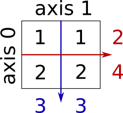
Sum by rows and by columns:

x = np.array([[1, 1], [2, 2]])
x

array([[1, 1],
       [2, 2]])

x.sum(axis=0)   # columns (first dimension)

array([3, 3])

x[:, 0].sum(), x[:, 1].sum()

(np.int64(3), np.int64(3))

x.sum(axis=1)   # rows (second dimension)

array([2, 4])

x[0, :].sum(), x[1, :].sum()

(np.int64(2), np.int64(4))

Here is the same idea in higher dimensions:

rng = np.random.default_rng(27446968)
x = rng.random((2, 2, 2))
x.sum(axis=2)[0, 1]

np.float64(0.7341517644004746)

x[0, 1, :].sum()

np.float64(0.7341517644004746)

Other reductions

These work the same way (and take axis=)

Extrema

x = np.array([1, 3, 2])
x.min()

np.int64(1)

x.max()

np.int64(3)

x.argmin()  # index of minimum

np.int64(0)

x.argmax()  # index of maximum

np.int64(1)

Logical operations

np.all([True, True, False])

np.False_

np.any([True, True, False])

np.True_

This can be used for array comparisons:

a = np.zeros((100, 100))
np.any(a != 0)

np.False_

np.all(a == a)

np.True_

a = np.array([1, 2, 3, 2])
b = np.array([2, 2, 3, 2])
c = np.array([6, 4, 4, 5])
((a <= b) & (b <= c)).all()

np.True_

Statistics:

x = np.array([1, 2, 3, 1])
y = np.array([[1, 2, 3], [5, 6, 1]])
x.mean()

np.float64(1.75)

np.median(x)

np.float64(1.5)

np.median(y, axis=-1) # last axis

array([2., 5.])

x.std()          # full population standard dev.

np.float64(0.82915619758885)

… and many more (best to learn as you go).

Exercise 17

Given there is a sum, what other function might you expect to see? What is the difference between sum and cumsum?

Worked Example: diffusion using a random walk algorithm

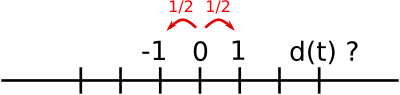
Let us consider a simple 1D random walk process: at each time step a walker jumps right or left with equal probability.

We are interested in finding the typical distance from the origin of a random walker after t left or right jumps? We are going to simulate many “walkers” to find this law, and we are going to do so using array computing tricks: we are going to create a 2D array with the “stories” (each walker has a story) in one direction, and the time in the other:

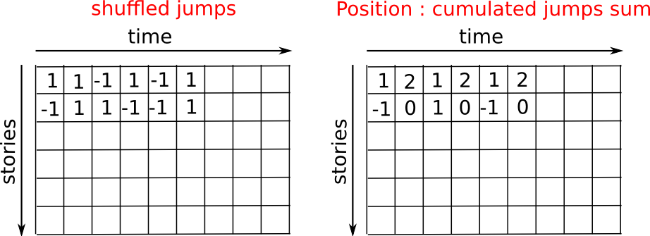
n_stories = 1000 # number of walkers
t_max = 200      # time during which we follow the walker

We randomly choose all the steps 1 or -1 of the walk:

t = np.arange(t_max)
rng = np.random.default_rng()
steps = 2 * rng.integers(0, 1 + 1, (n_stories, t_max)) - 1 # +1 because the high value is exclusive
np.unique(steps) # Verification: all steps are 1 or -1

array([-1,  1])

We build the walks by summing steps along the time:

positions = np.cumsum(steps, axis=1) # axis = 1: dimension of time
sq_distance = positions**2

We get the mean in the axis of the stories:

mean_sq_distance = np.mean(sq_distance, axis=0)

Plot the results:

plt.figure(figsize=(4, 3))
plt.plot(t, np.sqrt(mean_sq_distance), 'g.', t, np.sqrt(t), 'y-')
plt.xlabel(r"$t$")
plt.ylabel(r"$\sqrt{\langle (\delta x)^2 \rangle}$")
plt.tight_layout() # provide sufficient space for labels

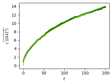
We find a well-known result in physics: the Root Mean Square (RMS) distance grows as the square root of the time!

Interim summary and exercises

Operation type	Numpy functions
arithmetic	sum, prod, mean, std
Extrema	min, max
logical	all, any

Also, recall the axis argument to select the dimension over which an operation will be applied:

arr = np.array([[99, 12], [11, 2]])
arr

array([[99, 12],
       [11,  2]])

# Without axis=, operation applied over whole (flatted, 1D) array.
np.min(arr)

np.int64(2)

# Operate along first axis (rows).
np.min(arr, axis=0)

array([11,  2])

# Operate along second axis (columns).
np.min(arr, axis=1)

array([12,  2])

Exercise 18

We load an array from a text file:

an_array = np.loadtxt('data/an_array.txt')

1. Verify if all elements in an array are equal to 1:

2. Verify if any elements in an array are equal to 1

3. Compute mean and standard deviation.

4. Challenge: write a function my_std that computes the standard deviation of the elements in the array, where you are only allowed to use np.sum from Numpy in your function. Check your function returns a value close to that from np.std (use np.allclose for that check).

Solution to Exercise 18

# 1. Verify if all elements in `an array` are equal to 1:
np.all(an_array == 1)

# 2. Verify if any elements in an array are equal to 1
np.any(an_array == 1)

# 3. Compute mean and standard deviation.
print('Mean', np.mean(an_array))
print('STD', np.std(an_array))

Mean 4.025
STD 2.1850343246731843

# 4. Challenge: write a function `my_std` that computes the standard deviation
# of the elements in the array, where you are only allowed to use `np.sum` from
# Numpy in your function.

def my_std(a):
    n = a.size
    m = np.sum(a) / n
    return np.sqrt(np.sum((a - m) ** 2) / n)

# Check we get the same answers from our function as for Numpy.
assert np.allclose(my_std(an_array), np.std(an_array))
assert np.allclose(my_std(an_array.ravel()), np.std(an_array))

rng = np.random.default_rng()
for i in range(10):
    another_array = rng.uniform(size=(10, 4))
    assert np.allclose(my_std(another_array), np.std(another_array))

Broadcasting

• Basic operations on numpy arrays (addition, etc.) are elementwise

• This works on arrays of the same size.

• Nevertheless , it’s also possible to do operations on arrays of different sizes if NumPy can transform these arrays so that they all have the same size: this conversion is called broadcasting.

The image below gives an example of broadcasting:

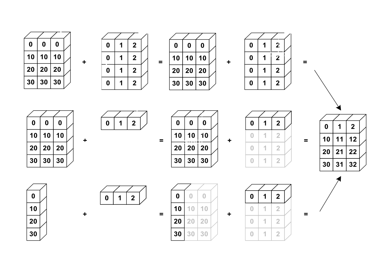
Let’s verify:

a = np.tile(np.arange(0, 40, 10), (3, 1)).T
a

array([[ 0,  0,  0],
       [10, 10, 10],
       [20, 20, 20],
       [30, 30, 30]])

b = np.array([0, 1, 2])
a + b

array([[ 0,  1,  2],
       [10, 11, 12],
       [20, 21, 22],
       [30, 31, 32]])

We have already used broadcasting without knowing it!:

a = np.ones((4, 5))
a[0] = 2  # we assign an array of dimension 0 to an array of dimension 1
a

array([[2., 2., 2., 2., 2.],
       [1., 1., 1., 1., 1.],
       [1., 1., 1., 1., 1.],
       [1., 1., 1., 1., 1.]])

A useful trick:

a = np.arange(0, 40, 10)
a.shape

(4,)

a = a[:, np.newaxis]  # adds a new axis -> 2D array
a.shape

(4, 1)

a

array([[ 0],
       [10],
       [20],
       [30]])

a + b

array([[ 0,  1,  2],
       [10, 11, 12],
       [20, 21, 22],
       [30, 31, 32]])

Note

Broadcasting seems a bit magical, but it is actually quite natural to use it when we want to solve a problem whose output data is an array with more dimensions than input data.

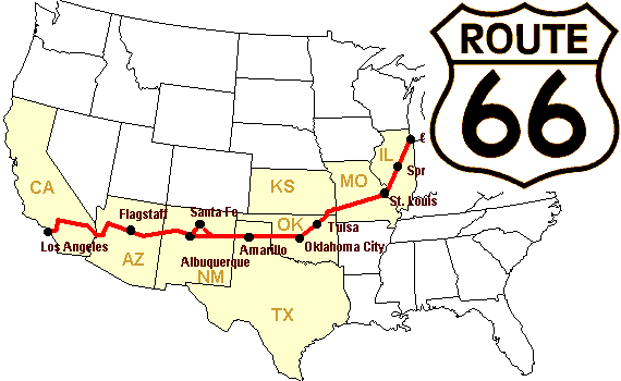
Worked Example: Broadcasting

Let’s construct an array of distances (in miles) between cities of Route 66: Chicago, Springfield, Saint-Louis, Tulsa, Oklahoma City, Amarillo, Santa Fe, Albuquerque, Flagstaff and Los Angeles.

mileposts = np.array([0, 198, 303, 736, 871, 1175, 1475, 1544,
       1913, 2448])
distance_array = np.abs(mileposts - mileposts[:, np.newaxis])
distance_array

array([[   0,  198,  303,  736,  871, 1175, 1475, 1544, 1913, 2448],
       [ 198,    0,  105,  538,  673,  977, 1277, 1346, 1715, 2250],
       [ 303,  105,    0,  433,  568,  872, 1172, 1241, 1610, 2145],
       [ 736,  538,  433,    0,  135,  439,  739,  808, 1177, 1712],
       [ 871,  673,  568,  135,    0,  304,  604,  673, 1042, 1577],
       [1175,  977,  872,  439,  304,    0,  300,  369,  738, 1273],
       [1475, 1277, 1172,  739,  604,  300,    0,   69,  438,  973],
       [1544, 1346, 1241,  808,  673,  369,   69,    0,  369,  904],
       [1913, 1715, 1610, 1177, 1042,  738,  438,  369,    0,  535],
       [2448, 2250, 2145, 1712, 1577, 1273,  973,  904,  535,    0]])

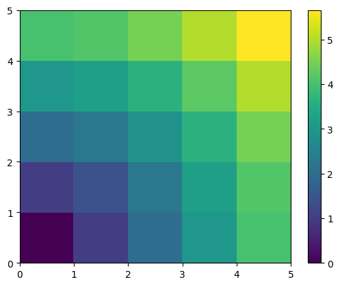
A lot of grid-based or network-based problems can also use broadcasting. For instance, if we want to compute the distance from the origin of points on a 5x5 grid, we can do

x, y = np.arange(5), np.arange(5)[:, np.newaxis]
distance = np.sqrt(x ** 2 + y ** 2)
distance

array([[0.        , 1.        , 2.        , 3.        , 4.        ],
       [1.        , 1.41421356, 2.23606798, 3.16227766, 4.12310563],
       [2.        , 2.23606798, 2.82842712, 3.60555128, 4.47213595],
       [3.        , 3.16227766, 3.60555128, 4.24264069, 5.        ],
       [4.        , 4.12310563, 4.47213595, 5.        , 5.65685425]])

Or in color:

plt.pcolor(distance)
plt.colorbar()

<matplotlib.colorbar.Colorbar at 0x11482f7d0>

Remark : the numpy.ogrid() function allows to directly create vectors x and y of the previous example, with two “significant dimensions”:

x, y = np.ogrid[0:5, 0:5]
x, y

(array([[0],
        [1],
        [2],
        [3],
        [4]]),
 array([[0, 1, 2, 3, 4]]))

x.shape, y.shape
distance = np.sqrt(x ** 2 + y ** 2)

So, np.ogrid is very useful as soon as we have to handle computations on a grid. On the other hand, np.mgrid directly provides matrices full of indices for cases where we can’t (or don’t want to) benefit from broadcasting:

x, y = np.mgrid[0:4, 0:4]
x

array([[0, 0, 0, 0],
       [1, 1, 1, 1],
       [2, 2, 2, 2],
       [3, 3, 3, 3]])

y

array([[0, 1, 2, 3],
       [0, 1, 2, 3],
       [0, 1, 2, 3],
       [0, 1, 2, 3]])

See also

Broadcasting: discussion of broadcasting in the Advanced NumPy chapter.

Array shape manipulation

Flattening

a = np.array([[1, 2, 3], [4, 5, 6]])
a.ravel()

array([1, 2, 3, 4, 5, 6])

a.T

array([[1, 4],
       [2, 5],
       [3, 6]])

a.T.ravel()

array([1, 4, 2, 5, 3, 6])

Higher dimensions: last dimensions ravel out “first”.

Reshaping

The inverse operation to flattening:

a.shape

(2, 3)

b = a.ravel()
b = b.reshape((2, 3))
b

array([[1, 2, 3],
       [4, 5, 6]])

Or,

a.reshape((2, -1))    # unspecified (-1) value is inferred

array([[1, 2, 3],
       [4, 5, 6]])

Warning

ndarray.reshape may return a view (cf help(np.reshape))), or copy

For example, consider:

b[0, 0] = 99
a

array([[99,  2,  3],
       [ 4,  5,  6]])

Beware: reshape may also return a copy!:

a = np.zeros((3, 2))
b = a.T.reshape(3*2)
b[0] = 9
a

array([[0., 0.],
       [0., 0.],
       [0., 0.]])

To understand this you need to learn more about the memory layout of a NumPy array.

Adding a dimension

Indexing with the np.newaxis object allows us to add an axis to an array (you have seen this already above in the broadcasting section):

z = np.array([1, 2, 3])
z

array([1, 2, 3])

z[:, np.newaxis]

array([[1],
       [2],
       [3]])

z[np.newaxis, :]

array([[1, 2, 3]])

Dimension shuffling

a = np.arange(4*3*2).reshape(4, 3, 2)
a.shape

(4, 3, 2)

a[0, 2, 1]

np.int64(5)

b = a.transpose(1, 2, 0)
b.shape

(3, 2, 4)

b[2, 1, 0]

np.int64(5)

Also creates a view:

b[2, 1, 0] = -1
a[0, 2, 1]

np.int64(-1)

Resizing

Size of an array can be changed with ndarray.resize:

a = np.arange(4)
a.resize((8,))
a

array([0, 1, 2, 3, 0, 0, 0, 0])

However, it must not be referred to somewhere else:

b = a
a.resize((4,))

---------------------------------------------------------------------------
ValueError                                Traceback (most recent call last)
Cell In[90], line 2
      1 b = a
----> 2 a.resize((4,))

ValueError: cannot resize an array that references or is referenced
by another array in this way.
Use the np.resize function or refcheck=False

Exercise 19

• Look at the docstring for reshape, especially the notes section which has some more information about copies and views.

• Use flatten as an alternative to ravel. What is the difference? (Hint: check which one returns a view and which a copy)

• Experiment with transpose for dimension shuffling.

Sorting data

Sorting along an axis:

a = np.array([[4, 3, 5], [1, 2, 1]])
b = np.sort(a, axis=1)
b

array([[3, 4, 5],
       [1, 1, 2]])

Note

Sorts each row separately!

In-place sort:

a.sort(axis=1)
a

array([[3, 4, 5],
       [1, 1, 2]])

Sorting with fancy indexing:

a = np.array([4, 3, 1, 2])
j = np.argsort(a)
j

array([2, 3, 1, 0])

a[j]

array([1, 2, 3, 4])

Finding minima and maxima:

a = np.array([4, 3, 1, 2])
j_max = np.argmax(a)
j_min = np.argmin(a)
j_max, j_min

(np.int64(0), np.int64(2))

Exercise 20

• Try both in-place and out-of-place sorting.

• Try creating arrays with different dtypes and sorting them.

• Use all or array_equal to check the results.

• Look at np.random.shuffle for a way to create sortable input quicker.

• Combine ravel, sort and reshape.

• Look at the axis keyword for sort and rewrite the previous exercise.

Summary

What do you need to know to get started?

• Know how to create arrays : array, arange, ones, zeros.

• Know the shape of the array with array.shape, then use slicing to obtain different views of the array: array[::2], etc. Adjust the shape of the array using reshape or flatten it with ravel.

• Obtain a subset of the elements of an array and/or modify their values with masks, with e.g.:

  a[a < 0] = 0
  

• Know miscellaneous operations on arrays, such as finding the mean or max (array.max(), array.mean()). No need to retain everything, but have the reflex to search in the documentation (online docs, help())!!

• For advanced use: master the indexing with arrays of integers, as well as broadcasting. Know more NumPy functions to handle various array operations.

Quick read

If you want to do a first quick pass through the Scientific Python Lectures to learn the ecosystem, you can directly skip to the next chapter: Matplotlib: plotting.

The remainder of this chapter is not necessary to follow the rest of the intro part. But be sure to come back and finish this chapter, as well as to do some more exercises.