
The NumPy array object#
What are NumPy and NumPy arrays?#
NumPy arrays#
NumPy provides:
An extension package to Python for multi-dimensional arrays.
An implementation that is closer to hardware (efficiency).
Package designed for scientific computation (convenience).
An implementation of array oriented computing.
import numpy as np

a = np.array([0, 1, 2, 3])
a
array([0, 1, 2, 3])
Note
For example, An array containing:
values of an experiment/simulation at discrete time steps
signal recorded by a measurement device, e.g. sound wave
pixels of an image, grey-level or colour
3-D data measured at different X-Y-Z positions, e.g. MRI scan
…
Why it is useful: Memory-efficient container that provides fast numerical operations.
L = range(1000)
%timeit [i**2 for i in L]
71.9 μs ± 176 ns per loop (mean ± std. dev. of 7 runs, 10,000 loops each)
a = np.arange(1000)
%timeit a**2
851 ns ± 13.4 ns per loop (mean ± std. dev. of 7 runs, 1,000,000 loops each)
NumPy Reference documentation#
On the web:
Interactive help:
In [5]: np.array?
String Form:<built-in function array>
Docstring:
array(object, dtype=None, copy=True, order=None, subok=False, ndmin=0, ...
You can also use the Python builtin help command to show the docstring for a function:
help(np.array)
Help on built-in function array in module numpy:

array(...)
    array(object, dtype=None, *, copy=True, order='K', subok=False, ndmin=0,
          like=None)

    Create an array.

    Parameters
    ----------
    object : array_like
        An array, any object exposing the array interface, an object whose
        ``__array__`` method returns an array, or any (nested) sequence.
        If object is a scalar, a 0-dimensional array containing object is
        returned.
    dtype : data-type, optional
        The desired data-type for the array. If not given, NumPy will try to use
        a default ``dtype`` that can represent the values (by applying promotion
        rules when necessary.)
    copy : bool, optional
        If ``True`` (default), then the array data is copied. If ``None``,
        a copy will only be made if ``__array__`` returns a copy, if obj is
        a nested sequence, or if a copy is needed to satisfy any of the other
        requirements (``dtype``, ``order``, etc.). Note that any copy of
        the data is shallow, i.e., for arrays with object dtype, the new
        array will point to the same objects. See Examples for `ndarray.copy`.
        For ``False`` it raises a ``ValueError`` if a copy cannot be avoided.
        Default: ``True``.
    order : {'K', 'A', 'C', 'F'}, optional
        Specify the memory layout of the array. If object is not an array, the
        newly created array will be in C order (row major) unless 'F' is
        specified, in which case it will be in Fortran order (column major).
        If object is an array the following holds.

        ===== ========= ===================================================
        order  no copy                     copy=True
        ===== ========= ===================================================
        'K'   unchanged F & C order preserved, otherwise most similar order
        'A'   unchanged F order if input is F and not C, otherwise C order
        'C'   C order   C order
        'F'   F order   F order
        ===== ========= ===================================================

        When ``copy=None`` and a copy is made for other reasons, the result is
        the same as if ``copy=True``, with some exceptions for 'A', see the
        Notes section. The default order is 'K'.
    subok : bool, optional
        If True, then sub-classes will be passed-through, otherwise
        the returned array will be forced to be a base-class array (default).
    ndmin : int, optional
        Specifies the minimum number of dimensions that the resulting
        array should have.  Ones will be prepended to the shape as
        needed to meet this requirement.
    like : array_like, optional
        Reference object to allow the creation of arrays which are not
        NumPy arrays. If an array-like passed in as ``like`` supports
        the ``__array_function__`` protocol, the result will be defined
        by it. In this case, it ensures the creation of an array object
        compatible with that passed in via this argument.

        .. versionadded:: 1.20.0

    Returns
    -------
    out : ndarray
        An array object satisfying the specified requirements.

    See Also
    --------
    empty_like : Return an empty array with shape and type of input.
    ones_like : Return an array of ones with shape and type of input.
    zeros_like : Return an array of zeros with shape and type of input.
    full_like : Return a new array with shape of input filled with value.
    empty : Return a new uninitialized array.
    ones : Return a new array setting values to one.
    zeros : Return a new array setting values to zero.
    full : Return a new array of given shape filled with value.
    copy: Return an array copy of the given object.


    Notes
    -----
    When order is 'A' and ``object`` is an array in neither 'C' nor 'F' order,
    and a copy is forced by a change in dtype, then the order of the result is
    not necessarily 'C' as expected. This is likely a bug.

    Examples
    --------
    >>> import numpy as np
    >>> np.array([1, 2, 3])
    array([1, 2, 3])

    Upcasting:

    >>> np.array([1, 2, 3.0])
    array([ 1.,  2.,  3.])

    More than one dimension:

    >>> np.array([[1, 2], [3, 4]])
    array([[1, 2],
           [3, 4]])

    Minimum dimensions 2:

    >>> np.array([1, 2, 3], ndmin=2)
    array([[1, 2, 3]])

    Type provided:

    >>> np.array([1, 2, 3], dtype=complex)
    array([ 1.+0.j,  2.+0.j,  3.+0.j])

    Data-type consisting of more than one element:

    >>> x = np.array([(1,2),(3,4)],dtype=[('a','<i4'),('b','<i4')])
    >>> x['a']
    array([1, 3], dtype=int32)

    Creating an array from sub-classes:

    >>> np.array(np.asmatrix('1 2; 3 4'))
    array([[1, 2],
           [3, 4]])

    >>> np.array(np.asmatrix('1 2; 3 4'), subok=True)
    matrix([[1, 2],
            [3, 4]])
Looking for something:#
In [6]: np.con*?
np.concatenate
np.conj
np.conjugate
np.convolve
Import conventions#
The recommended convention to import NumPy is:
import numpy as np
Creating arrays#
Manual construction of arrays#
1-D:
a = np.array([0, 1, 2, 3])
a
array([0, 1, 2, 3])
a.ndim
1
a.shape
(4,)
len(a)
4
2-D, 3-D, …:
b = np.array([[0, 1, 2], [3, 4, 5]])    # 2 x 3 array
b
array([[0, 1, 2],
       [3, 4, 5]])
b.ndim
2
b.shape
(2, 3)
len(b) # returns the size of the first dimension
2
c = np.array([[[1], [2]], [[3], [4]]])
c
array([[[1],
        [2]],

       [[3],
        [4]]])
c.shape
(2, 2, 1)
Exercise 7
Create a simple two dimensional array. First, redo the examples from above. And then create your own: how about odd numbers counting backwards on the first row, and even numbers on the second?
Use the functions
len(),numpy.shape()on these arrays. How do they relate to each other? And to thendimattribute of the arrays?
Functions for creating arrays#
Note
In practice, we rarely enter items one by one…
Evenly spaced:
a = np.arange(10) # 0 .. n-1  (!)
a
array([0, 1, 2, 3, 4, 5, 6, 7, 8, 9])
b = np.arange(1, 9, 2) # start, end (exclusive), step
b
array([1, 3, 5, 7])
— or by number of points
c = np.linspace(0, 1, 6)   # start, end, num-points
c
array([0. , 0.2, 0.4, 0.6, 0.8, 1. ])
d = np.linspace(0, 1, 5, endpoint=False)
d
array([0. , 0.2, 0.4, 0.6, 0.8])
Common arrays
a = np.ones((3, 3))  # reminder: (3, 3) is a tuple
a
array([[1., 1., 1.],
       [1., 1., 1.],
       [1., 1., 1.]])
b = np.zeros((2, 2))
b
array([[0., 0.],
       [0., 0.]])
c = np.eye(3)
c
array([[1., 0., 0.],
       [0., 1., 0.],
       [0., 0., 1.]])
d = np.diag(np.array([1, 2, 3, 4]))
d
array([[1, 0, 0, 0],
       [0, 2, 0, 0],
       [0, 0, 3, 0],
       [0, 0, 0, 4]])
numpy.random: random numbers (Mersenne Twister PRNG):
rng = np.random.default_rng(27446968)
a = rng.random(4)       # uniform in [0, 1]
a
array([0.64613018, 0.48984931, 0.50851229, 0.22563948])
b = rng.standard_normal(4)      # Gaussian
b
array([-0.38250769, -0.61536465, 0.98131732, 0.59353096])
Exercise 8
Experiment with
arange,linspace,ones,zeros,eyeanddiag.Create different kinds of arrays with random numbers.
Try setting the seed before creating an array with random values.
Look at the function
np.empty. What does it do? When might this be useful?
Exercise 9
construct an array containing: 1 2 3 4 5
construct an array containing: -5, -4, -3, -2, -1
Construct: 2 4 6 8
Construct 15 equispaced numbers in range [0, 10]
Solution to Exercise 9
np.arange(1, 6)
array([1, 2, 3, 4, 5])
np.arange(-5, 0)
array([-5, -4, -3, -2, -1])
np.arange(2, 10, 2)
array([2, 4, 6, 8])
np.linspace(0, 10, 15)
array([ 0.        ,  0.71428571,  1.42857143,  2.14285714,  2.85714286,
        3.57142857,  4.28571429,  5.        ,  5.71428571,  6.42857143,
        7.14285714,  7.85714286,  8.57142857,  9.28571429, 10.        ])
Basic data types#
You may have noticed that, in some instances, array elements are displayed with
a trailing dot (e.g. 2. vs 2). This is due to a difference in the
data-type used:
a = np.array([1, 2, 3])
a.dtype
dtype('int64')
b = np.array([1., 2., 3.])
b.dtype
dtype('float64')
Note
Different data-types allow us to store data more compactly in memory, but most of the time we simply work with floating point numbers. Note that, in the example above, NumPy auto-detects the data-type from the input.
You can explicitly specify which data-type you want:
c = np.array([1, 2, 3], dtype=float)
c.dtype
dtype('float64')
The default data type is floating point:
a = np.ones((3, 3))
a.dtype
dtype('float64')
There are also other types:
Bool#
e = np.array([True, False, False, True])
e.dtype
dtype('bool')
Strings#
f = np.array(['Bonjour', 'Hello', 'Hallo'])
f.dtype     # <--- strings containing max. 7 letters
dtype('<U7')
Much more:#
int32int64uint32uint64…
Basic visualization#
Now that we have our first data arrays, we are going to visualize them.
Start by launching IPython:
$ ipython # or ipython3 depending on your install
Or the notebook:
$ jupyter notebook
If you are using IPython enable interactive plots with:
%matplotlib
Using matplotlib backend: module://matplotlib_inline.backend_inline
Interactive plots are enabled automatically in the Jupyter Notebook.
Matplotlib is a 2D plotting package. We can import its functions as below:
import matplotlib.pyplot as plt # the tidy way
And then use (note that you have to use show explicitly if you have not enabled interactive plots with %matplotlib):
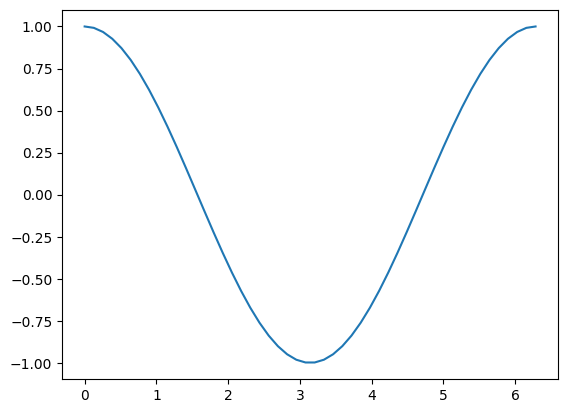
# Example data
x = np.linspace(0, 2 * np.pi)
y = np.cos(x)

plt.plot(x, y)       # line plot
plt.show()           # <-- shows the plot (not needed with interactive plots)
Or, if you have enabled interactive plots with %matplotlib:
plt.plot(x, y) # line plot
[<matplotlib.lines.Line2D at 0x1069c11f0>]
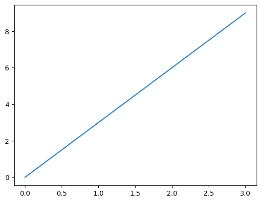
1D plotting:
x = np.linspace(0, 3, 20)
y = np.linspace(0, 9, 20)
plt.plot(x, y)       # line plot
[<matplotlib.lines.Line2D at 0x106a19760>]
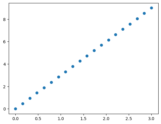
plt.plot(x, y, 'o') # dot plot
[<matplotlib.lines.Line2D at 0x106a75f70>]
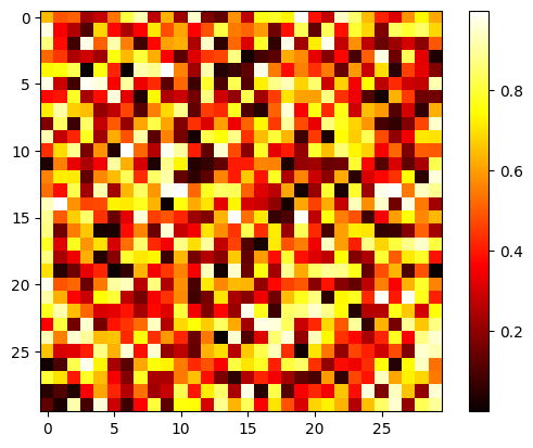
2D arrays (such as images):
rng = np.random.default_rng(27446968)
image = rng.random((30, 30))
plt.imshow(image, cmap=plt.cm.hot)
plt.colorbar()
<matplotlib.colorbar.Colorbar at 0x1069942c0>
See also
More in the: matplotlib chapter
Exercise 10
Plot some simple arrays: a cosine as a function of time and a 2D matrix.
Try using the
graycolormap on the 2D matrix.
Indexing and slicing#
The items of an array can be accessed and assigned to the same way as other Python sequences (e.g. lists):
a = np.arange(10)
a
array([0, 1, 2, 3, 4, 5, 6, 7, 8, 9])
a[0], a[2], a[-1]
(np.int64(0), np.int64(2), np.int64(9))
Warning
Indices begin at 0, like other Python sequences (and C/C++). In contrast, in Fortran or Matlab, indices begin at 1.
The usual python idiom for reversing a sequence is supported:
a[::-1]
array([9, 8, 7, 6, 5, 4, 3, 2, 1, 0])
For multidimensional arrays, indices are tuples of integers:
a = np.diag(np.arange(3))
a
array([[0, 0, 0],
       [0, 1, 0],
       [0, 0, 2]])
a[1, 1]
np.int64(1)
a[2, 1] = 10 # third line, second column
a
array([[ 0,  0,  0],
       [ 0,  1,  0],
       [ 0, 10,  2]])
a[1]
array([0, 1, 0])
Note
In 2D, the first dimension corresponds to rows, the second to columns.
for multidimensional
a,a[0]is interpreted by taking all elements in the unspecified dimensions.
Slicing: Arrays, like other Python sequences can also be sliced:
a = np.arange(10)
a
array([0, 1, 2, 3, 4, 5, 6, 7, 8, 9])
a[2:9:3] # [start:end:step]
array([2, 5, 8])
Note that the last index is not included! :
a[:4]
array([0, 1, 2, 3])
All three slice components are not required: by default, start is 0,
end is the last and step is 1:
a[1:3]
array([1, 2])
a[::2]
array([0, 2, 4, 6, 8])
a[3:]
array([3, 4, 5, 6, 7, 8, 9])
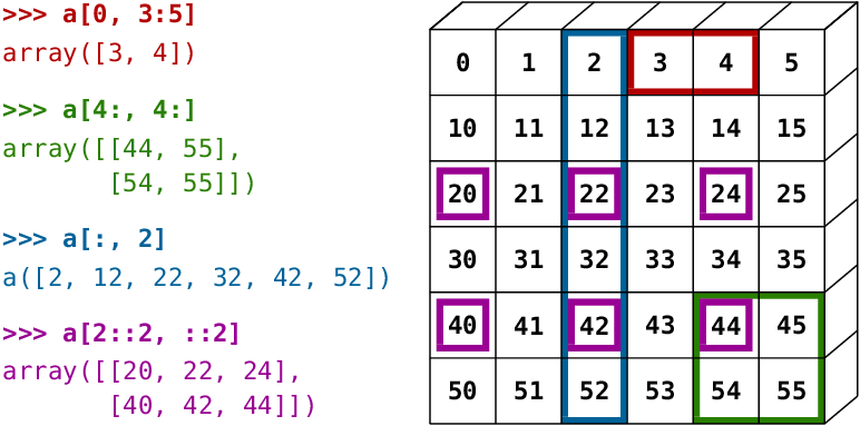
A small illustrated summary of NumPy indexing and slicing…
You can also combine assignment and slicing:
a = np.arange(10)
a[5:] = 10
a
array([ 0, 1, 2, 3, 4, 10, 10, 10, 10, 10])
b = np.arange(5)
a[5:] = b[::-1]
a
array([0, 1, 2, 3, 4, 4, 3, 2, 1, 0])
Exercise 11
Try the different flavours of slicing, using
start,endandstep: starting from a linspace, try to obtain odd numbers counting backwards, and even numbers counting forwards.Reproduce the slices in the diagram above. You may use the following expression to create the array:
np.arange(6) + np.arange(0, 51, 10)[:, np.newaxis]
Exercise 12
An exercise on array creation.
Create the following arrays (with correct data types):
[[1, 1, 1, 1],
 [1, 1, 1, 1],
 [1, 1, 1, 2],
 [1, 6, 1, 1]]

[[0., 0., 0., 0., 0.],
 [2., 0., 0., 0., 0.],
 [0., 3., 0., 0., 0.],
 [0., 0., 4., 0., 0.],
 [0., 0., 0., 5., 0.],
 [0., 0., 0., 0., 6.]]
Par on course: 3 statements for each.
Hint: Individual array elements can be accessed similarly to a list,
e.g. a[1] or a[1, 2].
Hint: Examine the docstring for diag.
Solution to Exercise 12
a = np.ones((4, 4), dtype=int)
a[3, 1] = 6
a[2, 3] = 2
a
array([[1, 1, 1, 1],
       [1, 1, 1, 1],
       [1, 1, 1, 2],
       [1, 6, 1, 1]])
b = np.zeros((6, 5))
b[1:] = np.diag(np.arange(2, 7))
b
array([[0., 0., 0., 0., 0.],
       [2., 0., 0., 0., 0.],
       [0., 3., 0., 0., 0.],
       [0., 0., 4., 0., 0.],
       [0., 0., 0., 5., 0.],
       [0., 0., 0., 0., 6.]])
Exercise 13
Exercise on tiling for array creation.
Skim through the documentation for np.tile, and use this function
to construct the array:
[[4, 3, 4, 3, 4, 3],
 [2, 1, 2, 1, 2, 1],
 [4, 3, 4, 3, 4, 3],
 [2, 1, 2, 1, 2, 1]]
Solution to Exercise 13
block = np.array([[4, 3], [2, 1]])
a = np.tile(block, (2, 3))
a
array([[4, 3, 4, 3, 4, 3],
       [2, 1, 2, 1, 2, 1],
       [4, 3, 4, 3, 4, 3],
       [2, 1, 2, 1, 2, 1]])
Copies and views#
A slicing operation creates a view on the original array, which is
just a way of accessing array data. Thus the original array is not
copied in memory. You can use np.may_share_memory() to check if two arrays
share the same memory block. Note however, that this uses heuristics and may
give you false positives.
When modifying the view, the original array is modified as well:
a = np.arange(10)
a
array([0, 1, 2, 3, 4, 5, 6, 7, 8, 9])
b = a[::2]
b
array([0, 2, 4, 6, 8])
np.may_share_memory(a, b)
True
b[0] = 12
b
array([12, 2, 4, 6, 8])
a # (!)
array([12, 1, 2, 3, 4, 5, 6, 7, 8, 9])
a = np.arange(10)
c = a[::2].copy()  # force a copy
c[0] = 12
a
array([0, 1, 2, 3, 4, 5, 6, 7, 8, 9])
np.may_share_memory(a, c)
False
This behavior can be surprising at first sight… but it allows to save both memory and time.
Worked example: Prime number sieve#
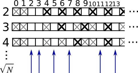
Compute prime numbers in 0–99, with a sieve
First — construct a shape (100,) boolean array is_prime, filled with True in
the beginning:
is_prime = np.ones((100,), dtype=bool)
Next, cross out 0 and 1 which are not primes:
is_prime[:2] = 0
For each integer j starting from 2, cross out its higher multiples:
N_max = int(np.sqrt(len(is_prime) - 1))
for j in range(2, N_max + 1):
    is_prime[2*j::j] = False
Skim through help(np.nonzero), and print the prime numbers
Follow-up:
Move the above code into a script file named
prime_sieve.pyRun it to check it works
Use the optimization suggested in the sieve of Eratosthenes:
Skip
jwhich are already known to not be primesThe first number to cross out is \(j^2\)
Fancy indexing#
Note
NumPy arrays can be indexed with slices, but also with boolean or integer arrays (masks). This method is called fancy indexing. It creates copies not views.
Using boolean masks#
rng = np.random.default_rng(27446968)
a = rng.integers(0, 21, 15)
a
array([ 3, 13, 12, 10, 10, 10, 18, 4, 8, 5, 6, 11, 12, 17, 3])
(a % 3 == 0)
array([ True, False,  True, False, False, False,  True, False, False,
       False,  True, False,  True, False,  True])
mask = (a % 3 == 0)
extract_from_a = a[mask] # or,  a[a%3==0]
extract_from_a           # extract a sub-array with the mask
array([ 3, 12, 18, 6, 12, 3])
Indexing with a mask can be very useful to assign a new value to a sub-array:
a[a % 3 == 0] = -1
a
array([-1, 13, -1, 10, 10, 10, -1, 4, 8, 5, -1, 11, -1, 17, -1])
Indexing with an array of integers#
a = np.arange(0, 100, 10)
a
array([ 0, 10, 20, 30, 40, 50, 60, 70, 80, 90])
Indexing can be done with an array of integers, where the same index is repeated several time:
a[[2, 3, 2, 4, 2]] # note: [2, 3, 2, 4, 2] is a Python list
array([20, 30, 20, 40, 20])
New values can be assigned with this kind of indexing:
a[[9, 7]] = -100
a
array([ 0, 10, 20, 30, 40, 50, 60, -100, 80, -100])
Tip
When a new array is created by indexing with an array of integers, the new array has the same shape as the array of integers:
a = np.arange(10)
idx = np.array([[3, 4], [9, 7]])
idx.shape
(2, 2)
a[idx]
array([[3, 4],
       [9, 7]])
The image below illustrates various fancy indexing applications
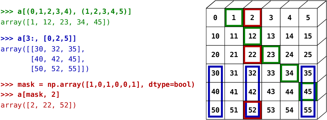
Exercise 14
Again, reproduce the fancy indexing shown in the diagram above.
Use fancy indexing on the left and array creation on the right to assign values into an array, for instance by setting parts of the array in the diagram above to zero.
We can even use fancy indexing and broadcasting at the same time:
a = np.arange(12).reshape(3,4)
a
array([[ 0,  1,  2,  3],
       [ 4,  5,  6,  7],
       [ 8,  9, 10, 11]])
i = np.array([[0, 1], [1, 2]])
a[i, 2]  # same as a[i, 2 * np.ones((2, 2), dtype=int)]
array([[ 2,  6],
       [ 6, 10]])