Some exercises

import numpy as np
import matplotlib.pyplot as plt

Array manipulations

Exercise 22

Form the 2-D array (without typing it in explicitly)

[[1,  6, 11],
 [2,  7, 12],
 [3,  8, 13],
 [4,  9, 14],
 [5, 10, 15]]

and generate a new array containing its 2nd and 4th rows.

Divide each column of the array

import numpy as np
a = np.arange(25).reshape(5, 5)

elementwise with the array b = np.array([1., 5, 10, 15, 20]). (Hint: np.newaxis).

Harder one, random numbers

Generate a 10 x 3 array of random numbers (in range [0,1]). For each row, pick the number closest to 0.5.

• Use abs and argmin to find the column j closest for each row.

• Use fancy indexing to extract the numbers. (Hint: a[i,j] – the array i must contain the row numbers corresponding to stuff in j.)

Solution to Exercise 22

import numpy as np
from numpy import newaxis

# Part 1.

a = np.arange(1, 16).reshape(3, -1).T
print(a)

[[ 1  6 11]
 [ 2  7 12]
 [ 3  8 13]
 [ 4  9 14]
 [ 5 10 15]]

Picture manipulation: Framing a Face

Let’s do some manipulations on NumPy arrays by starting with an image of a raccoon. scipy provides a 2D array of this image with the scipy.datasets.face function:

import scipy as sp
face = sp.datasets.face(gray=True)  # 2D grayscale image

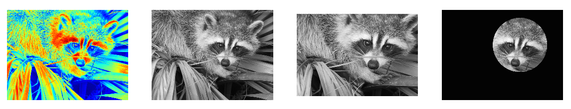
Here are a few images we will be able to obtain with our manipulations: use different colormaps, crop the image, change some parts of the image.

Let’s use the imshow function of matplotlib to display the image.

import matplotlib.pyplot as plt
face = sp.datasets.face(gray=True)
plt.imshow(face)

<matplotlib.image.AxesImage at 0x10d4b5970>

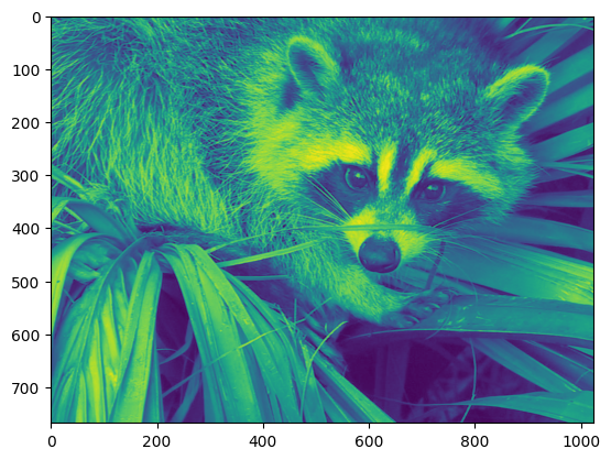
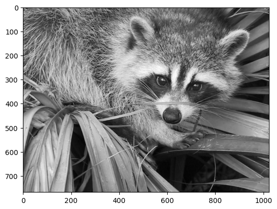
The face is displayed in false colors. A colormap must be specified for it to be displayed in grey.

plt.imshow(face, cmap=plt.cm.gray)

<matplotlib.image.AxesImage at 0x10f3ae3c0>

Narrow centering

Create an array of the image with a narrower centering; remove 100 pixels from all the borders of the image. To check the result, display this new array with imshow.

crop_face = face[100:-100, 100:-100]

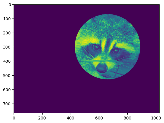
Frame face

We will now frame the face with a black locket. For this, we need to create a mask corresponding to the pixels we want to be black. The center of the face is around (660, 330), so we defined the mask by this condition `(y-300)**2

• (x-660)**2`

sy, sx = face.shape
y, x = np.ogrid[0:sy, 0:sx] # x and y indices of pixels
y.shape, x.shape

((768, 1), (1, 1024))

centerx, centery = (660, 300) # center of the image
mask = ((y - centery)**2 + (x - centerx)**2) > 230**2 # circle

then we assign the value 0 to the pixels of the image corresponding to the mask. The syntax is extremely simple and intuitive:

face[mask] = 0
plt.imshow(face)

<matplotlib.image.AxesImage at 0x10f58d0a0>

Follow-up:

• copy all instructions of this exercise in a script called : face_locket.py then execute this script in IPython with %run face_locket.py.

• Change the circle to an ellipsoid.

Data statistics

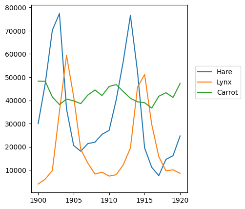
The data in populations.txt describes the populations of hares and lynxes (and carrots) in northern Canada during 20 years:

data = np.loadtxt('data/populations.txt')
year, hares, lynxes, carrots = data.T  # trick: columns to variables

import matplotlib.pyplot as plt

plt.axes([0.2, 0.1, 0.5, 0.8])
plt.plot(year, hares, year, lynxes, year, carrots)
plt.legend(('Hare', 'Lynx', 'Carrot'), loc=(1.05, 0.5))

<matplotlib.legend.Legend at 0x10f2b7920>

Exercise 23

Compute and print, based on the data in populations.txt…

1. The mean and std of the populations of each species for the years in the period.

2. Which year each species had the largest population.

3. Which species has the largest population for each year. (Hint: argsort & fancy indexing of np.array(['H', 'L', 'C']))

4. Which years any of the populations is above 50000. (Hint: comparisons and np.any)

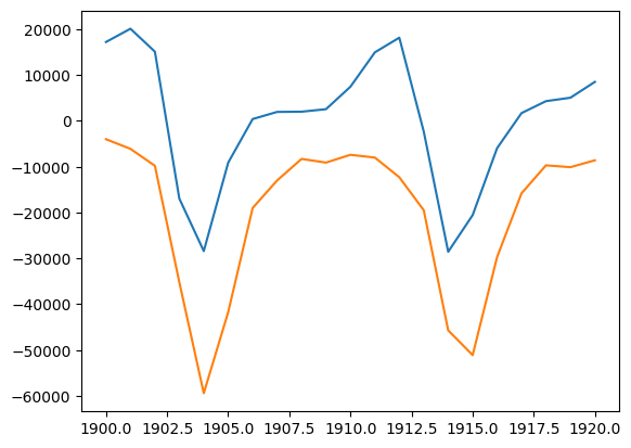
5. The top 2 years for each species when they had the lowest populations. (Hint: argsort, fancy indexing)

6. Compare (plot) the change in hare population (see help(np.gradient)) and the number of lynxes. Check correlation (see help(np.corrcoef)).

… all without for-loops.

Solution to Exercise 23

import numpy as np

data = np.loadtxt("data/populations.txt")
year, hares, lynxes, carrots = data.T
populations = data[:, 1:]

print("       Hares, Lynxes, Carrots")
print("Mean:", populations.mean(axis=0))
print("Std:", populations.std(axis=0))

j_max_years = np.argmax(populations, axis=0)
print("Max. year:", year[j_max_years])

max_species = np.argmax(populations, axis=1)
species = np.array(["Hare", "Lynx", "Carrot"])
print("Max species:")
print(year)
print(species[max_species])

above_50000 = np.any(populations > 50000, axis=1)
print("Any above 50000:", year[above_50000])

j_top_2 = np.argsort(populations, axis=0)[:2]
print("Top 2 years with lowest populations for each:")
print(year[j_top_2])

hare_grad = np.gradient(hares, 1.0)
print("diff(Hares) vs. Lynxes correlation", np.corrcoef(hare_grad, lynxes)[0, 1])

import matplotlib.pyplot as plt

plt.plot(year, hare_grad, year, -lynxes)
plt.savefig("plot.png")

       Hares, Lynxes, Carrots
Mean: [34080.95238095 20166.66666667 42400.        ]
Std: [20897.90645809 16254.59153691  3322.50622558]
Max. year: [1903. 1904. 1900.]
Max species:
[1900. 1901. 1902. 1903. 1904. 1905. 1906. 1907. 1908. 1909. 1910. 1911.
 1912. 1913. 1914. 1915. 1916. 1917. 1918. 1919. 1920.]
['Carrot' 'Carrot' 'Hare' 'Hare' 'Lynx' 'Lynx' 'Carrot' 'Carrot' 'Carrot'
 'Carrot' 'Carrot' 'Carrot' 'Hare' 'Hare' 'Hare' 'Lynx' 'Carrot' 'Carrot'
 'Carrot' 'Carrot' 'Carrot']
Any above 50000: [1902. 1903. 1904. 1912. 1913. 1914. 1915.]
Top 2 years with lowest populations for each:
[[1917. 1900. 1916.]
 [1916. 1901. 1903.]]
diff(Hares) vs. Lynxes correlation -0.917924848031534

Crude integral approximations

Exercise 24

Write a function f(a, b, c) that returns \(a^b - c\). Form a 24x12x6 array containing its values in parameter ranges [0,1] x [0,1] x [0,1].

Approximate the 3-d integral

\[ \int_0^1\int_0^1\int_0^1(a^b-c)da\,db\,dc \]

over this volume with the mean. The exact result is: \(\ln 2 - \frac{1}{2}\approx0.1931\ldots\) — what is your relative error?

(Hints: use elementwise operations and broadcasting. You can make np.ogrid give a number of points in given range with np.ogrid[0:1:20j].)

Reminder Python functions:

def f(a, b, c):
    return some_result

Solution to Exercise 24

import numpy as np
from numpy import newaxis


def f(a, b, c):
    return a**b - c


a = np.linspace(0, 1, 24)
b = np.linspace(0, 1, 12)
c = np.linspace(0, 1, 6)

samples = f(a[:, newaxis, newaxis], b[newaxis, :, newaxis], c[newaxis, newaxis, :])

# or,
#
# a, b, c = np.ogrid[0:1:24j, 0:1:12j, 0:1:6j]
# samples = f(a, b, c)

integral = samples.mean()

print("Approximation:", integral)
print("Exact:", np.log(2) - 0.5)

Approximation: 0.1888423460296792
Exact: 0.1931471805599453

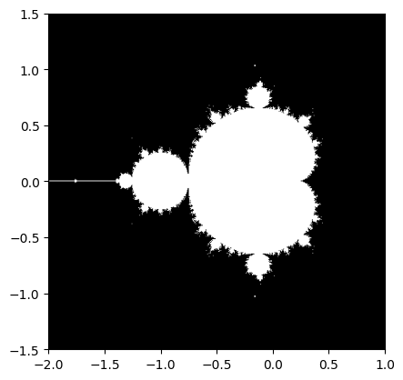
Mandelbrot set

Exercise 25

Write a script that computes the Mandelbrot fractal. The Mandelbrot iteration:

N_max = 50
some_threshold = 50

c = x + 1j*y

z = 0
for j in range(N_max):
    z = z**2 + c

/var/folders/hd/rfxyn9gx4bl39bvwzrgn3rtr0000gn/T/ipykernel_91679/585550489.py:8: RuntimeWarning: overflow encountered in square
  z = z**2 + c
/var/folders/hd/rfxyn9gx4bl39bvwzrgn3rtr0000gn/T/ipykernel_91679/585550489.py:8: RuntimeWarning: invalid value encountered in square
  z = z**2 + c

Point (x, y) belongs to the Mandelbrot set if \(|z|\) < some_threshold.

Do this computation by:

Show code cell source

Hide code cell source

mask = np.ones((3, 3))

1. Construct a grid of c = x + 1j*y values in range [-2, 1] x [-1.5, 1.5]

2. Do the iteration

3. Form the 2-d boolean mask indicating which points are in the set

4. Save the result to an image with:

   import matplotlib.pyplot as plt
   plt.imshow(mask.T, extent=[-2, 1, -1.5, 1.5])
   plt.gray()
   plt.savefig('mandelbrot.png')
   

Solution to Exercise 25

import numpy as np
import matplotlib.pyplot as plt
from numpy import newaxis


def compute_mandelbrot(N_max, some_threshold, nx, ny):
    # A grid of c-values
    x = np.linspace(-2, 1, nx)
    y = np.linspace(-1.5, 1.5, ny)

    c = x[:, newaxis] + 1j * y[newaxis, :]

    # Mandelbrot iteration

    z = c
    for j in range(N_max):
        z = z**2 + c

    mandelbrot_set = abs(z) < some_threshold

    return mandelbrot_set

# Save

mandelbrot_set = compute_mandelbrot(50, 50.0, 601, 401)

plt.imshow(mandelbrot_set.T, extent=[-2, 1, -1.5, 1.5])  # type: ignore[arg-type]
plt.gray()
plt.savefig("mandelbrot.png")

/var/folders/hd/rfxyn9gx4bl39bvwzrgn3rtr0000gn/T/ipykernel_91679/2370088976.py:17: RuntimeWarning: overflow encountered in square
  z = z**2 + c
/var/folders/hd/rfxyn9gx4bl39bvwzrgn3rtr0000gn/T/ipykernel_91679/2370088976.py:17: RuntimeWarning: invalid value encountered in square
  z = z**2 + c

Markov chain

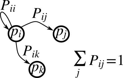
Exercise 26

Markov chain transition matrix P, and probability distribution on the states p:

1. 0 <= P[i,j] <= 1: probability to go from state i to state j

2. Transition rule: \(p_{new} = P^T p_{old}\)

3. all(sum(P, axis=1) == 1), p.sum() == 1: normalization

Write a script that works with 5 states, and:

• Constructs a random matrix, and normalizes each row so that it is a transition matrix.

• Starts from a random (normalized) probability distribution p and takes 50 steps => p_50

• Computes the stationary distribution: the eigenvector of P.T with eigenvalue 1 (numerically: closest to 1) => p_stationary

  Remember to normalize the eigenvector — I didn’t…

• Checks if p_50 and p_stationary are equal to tolerance 1e-5

Toolbox: np.random, @, np.linalg.eig, reductions, abs(), argmin, comparisons, all, np.linalg.norm, etc.

Solution to Exercise 26

Solution to Markov chain exercise.

import numpy as np

rng = np.random.default_rng(27446968)

n_states = 5
n_steps = 50
tolerance = 1e-5

# Random transition matrix and state vector
P = rng.random(size=(n_states, n_states))
p = rng.random(n_states)

# Normalize rows in P
P /= P.sum(axis=1)[:, np.newaxis]

# Normalize p
p /= p.sum()

# Take steps
for k in range(n_steps):
    p = P.T @ p

p_50 = p
print(p_50)

# Compute stationary state
w, v = np.linalg.eig(P.T)

j_stationary = np.argmin(abs(w - 1.0))
p_stationary = v[:, j_stationary].real
p_stationary /= p_stationary.sum()
print(p_stationary)

# Compare
if all(abs(p_50 - p_stationary) < tolerance):
    print("Tolerance satisfied in infty-norm")

if np.linalg.norm(p_50 - p_stationary) < tolerance:
    print("Tolerance satisfied in 2-norm")

[0.15219309 0.25577972 0.22811916 0.14261754 0.22129049]
[0.15219309 0.25577972 0.22811916 0.14261754 0.22129049]
Tolerance satisfied in infty-norm
Tolerance satisfied in 2-norm