Linear System Solvers#
sparse matrix/eigenvalue problem solvers live in
scipy.sparse.linalgthe submodules:
dsolve: direct factorization methods for solving linear systemsisolve: iterative methods for solving linear systemseigen: sparse eigenvalue problem solvers
All solvers are accessible from:
import scipy as sp
sp.sparse.linalg.__all__
['ArpackError',
 'ArpackNoConvergence',
 'LaplacianNd',
 'LinearOperator',
 'MatrixRankWarning',
 'SuperLU',
 'aslinearoperator',
 'bicg',
 'bicgstab',
 'cg',
 'cgs',
 'dsolve',
 'eigen',
 'eigs',
 'eigsh',
 'expm',
 'expm_multiply',
 'factorized',
 'gcrotmk',
 'gmres',
 'interface',
 'inv',
 'is_sptriangular',
 'isolve',
 'lgmres',
 'lobpcg',
 'lsmr',
 'lsqr',
 'matfuncs',
 'matrix_power',
 'minres',
 'norm',
 'onenormest',
 'qmr',
 'spbandwidth',
 'spilu',
 'splu',
 'spsolve',
 'spsolve_triangular',
 'svds',
 'tfqmr',
 'use_solver']
Sparse Direct Solvers#
default solver: SuperLU
included in SciPy
real and complex systems
both single and double precision
optional: umfpack
real and complex systems
double precision only
recommended for performance
wrappers now live in
scikits.umfpackcheck-out the new
scikits.suitesparseby Nathaniel Smith
Examples#
Import the whole module, and see its docstring:
help(sp.sparse.linalg.spsolve)
Help on function spsolve in module scipy.sparse.linalg._dsolve.linsolve:

spsolve(A, b, permc_spec=None, use_umfpack=True)
    Solve the sparse linear system Ax=b, where b may be a vector or a matrix.

    Parameters
    ----------
    A : ndarray or sparse array or matrix
        The square matrix A will be converted into CSC or CSR form
    b : ndarray or sparse array or matrix
        The matrix or vector representing the right hand side of the equation.
        If a vector, b.shape must be (n,) or (n, 1).
    permc_spec : str, optional
        How to permute the columns of the matrix for sparsity preservation.
        (default: 'COLAMD')

        - ``NATURAL``: natural ordering.
        - ``MMD_ATA``: minimum degree ordering on the structure of A^T A.
        - ``MMD_AT_PLUS_A``: minimum degree ordering on the structure of A^T+A.
        - ``COLAMD``: approximate minimum degree column ordering [1]_, [2]_.

    use_umfpack : bool, optional
        if True (default) then use UMFPACK for the solution [3]_, [4]_, [5]_,
        [6]_ . This is only referenced if b is a vector and
        ``scikits.umfpack`` is installed.

    Returns
    -------
    x : ndarray or sparse array or matrix
        the solution of the sparse linear equation.
        If b is a vector, then x is a vector of size A.shape[1]
        If b is a matrix, then x is a matrix of size (A.shape[1], b.shape[1])

    Notes
    -----
    For solving the matrix expression AX = B, this solver assumes the resulting
    matrix X is sparse, as is often the case for very sparse inputs.  If the
    resulting X is dense, the construction of this sparse result will be
    relatively expensive.  In that case, consider converting A to a dense
    matrix and using scipy.linalg.solve or its variants.

    References
    ----------
    .. [1] T. A. Davis, J. R. Gilbert, S. Larimore, E. Ng, Algorithm 836:
           COLAMD, an approximate column minimum degree ordering algorithm,
           ACM Trans. on Mathematical Software, 30(3), 2004, pp. 377--380.
           :doi:`10.1145/1024074.1024080`

    .. [2] T. A. Davis, J. R. Gilbert, S. Larimore, E. Ng, A column approximate
           minimum degree ordering algorithm, ACM Trans. on Mathematical
           Software, 30(3), 2004, pp. 353--376. :doi:`10.1145/1024074.1024079`

    .. [3] T. A. Davis, Algorithm 832:  UMFPACK - an unsymmetric-pattern
           multifrontal method with a column pre-ordering strategy, ACM
           Trans. on Mathematical Software, 30(2), 2004, pp. 196--199.
           https://dl.acm.org/doi/abs/10.1145/992200.992206

    .. [4] T. A. Davis, A column pre-ordering strategy for the
           unsymmetric-pattern multifrontal method, ACM Trans.
           on Mathematical Software, 30(2), 2004, pp. 165--195.
           https://dl.acm.org/doi/abs/10.1145/992200.992205

    .. [5] T. A. Davis and I. S. Duff, A combined unifrontal/multifrontal
           method for unsymmetric sparse matrices, ACM Trans. on
           Mathematical Software, 25(1), 1999, pp. 1--19.
           https://doi.org/10.1145/305658.287640

    .. [6] T. A. Davis and I. S. Duff, An unsymmetric-pattern multifrontal
           method for sparse LU factorization, SIAM J. Matrix Analysis and
           Computations, 18(1), 1997, pp. 140--158.
           https://doi.org/10.1137/S0895479894246905T.


    Examples
    --------
    >>> import numpy as np
    >>> from scipy.sparse import csc_array
    >>> from scipy.sparse.linalg import spsolve
    >>> A = csc_array([[3, 2, 0], [1, -1, 0], [0, 5, 1]], dtype=float)
    >>> B = csc_array([[2, 0], [-1, 0], [2, 0]], dtype=float)
    >>> x = spsolve(A, B)
    >>> np.allclose(A.dot(x).toarray(), B.toarray())
    True
Both superlu and umfpack can be used (if the latter is installed) as follows.
Prepare a linear system:
import numpy as np
mtx = sp.sparse.spdiags([[1, 2, 3, 4, 5], [6, 5, 8, 9, 10]], [0, 1], 5, 5, "csc")
mtx.toarray()
array([[ 1,  5,  0,  0,  0],
       [ 0,  2,  8,  0,  0],
       [ 0,  0,  3,  9,  0],
       [ 0,  0,  0,  4, 10],
       [ 0,  0,  0,  0,  5]])
rhs = np.array([1, 2, 3, 4, 5], dtype=np.float32)
Solve as single precision real:
mtx1 = mtx.astype(np.float32)
x = sp.sparse.linalg.spsolve(mtx1, rhs, use_umfpack=False)
print(x)
[106. -21. 5.5 -1.5 1. ]
print("Error: %s" % (mtx1 * x - rhs))
Error: [0. 0. 0. 0. 0.]
Solve as double precision real:
mtx2 = mtx.astype(np.float64)
x = sp.sparse.linalg.spsolve(mtx2, rhs, use_umfpack=True)
print(x)
[106. -21. 5.5 -1.5 1. ]
print("Error: %s" % (mtx2 * x - rhs))
Error: [0. 0. 0. 0. 0.]
Solve as single precision complex:
mtx1 = mtx.astype(np.complex64)
x = sp.sparse.linalg.spsolve(mtx1, rhs, use_umfpack=False)
print(x)
[106. +0.j -21. +0.j 5.5+0.j -1.5+0.j 1. +0.j]
print("Error: %s" % (mtx1 * x - rhs))
Error: [0.+0.j 0.+0.j 0.+0.j 0.+0.j 0.+0.j]
Solve as double precision complex:
mtx2 = mtx.astype(np.complex128)
x = sp.sparse.linalg.spsolve(mtx2, rhs, use_umfpack=True)
print(x)
[106. +0.j -21. +0.j 5.5+0.j -1.5+0.j 1. +0.j]
print("Error: %s" % (mtx2 * x - rhs))
Error: [0.+0.j 0.+0.j 0.+0.j 0.+0.j 0.+0.j]
Iterative Solvers#
the
isolvemodule contains the following solvers:bicg(BIConjugate Gradient)bicgstab(BIConjugate Gradient STABilized)cg(Conjugate Gradient) - symmetric positive definite matrices onlycgs(Conjugate Gradient Squared)gmres(Generalized Minimal RESidual)minres(MINimum RESidual)qmr(Quasi-Minimal Residual)
Common Parameters#
mandatory:
A: The N-by-N matrix of the linear system.b: Right hand side of the linear system. Has shape (N,) or (N,1).
optional:
x0: Starting guess for the solution.tol: Relative tolerance to achieve before terminating.maxiter: Maximum number of iterations. Iteration will stop after maxiter steps even if the specified tolerance has not been achieved.M: Preconditioner for A. The preconditioner should approximate the inverse of A. Effective preconditioning dramatically improves the rate of convergence, which implies that fewer iterations are needed to reach a given error tolerance.callback: User-supplied function to call after each iteration. It is called ascallback(xk), wherexkis the current solution vector.
LinearOperator Class#
common interface for performing matrix vector products
useful abstraction that enables using dense and sparse matrices within the solvers, as well as matrix-free solutions
has
shapeandmatvec()(+ some optional parameters)
Here is an example:
import numpy as np
import scipy as sp

def mv(v):
    return np.array([2 * v[0], 3 * v[1]])
A = sp.sparse.linalg.LinearOperator((2, 2), matvec=mv)
A
<2x2 _CustomLinearOperator with dtype=int8>
A.matvec(np.ones(2))
array([2., 3.])
A * np.ones(2)
array([2., 3.])
A Few Notes on Preconditioning#
problem specific
often hard to develop
if not sure, try ILU
available in
scipy.sparse.linalgasspilu()
Eigenvalue Problem Solvers#
The eigen module#
arpack: a collection of Fortran77 subroutines designed to solve large scale eigenvalue problemslobpcg: (Locally Optimal Block Preconditioned Conjugate Gradient Method); * works very well in combination with PyAMGexample by Nathan Bell:
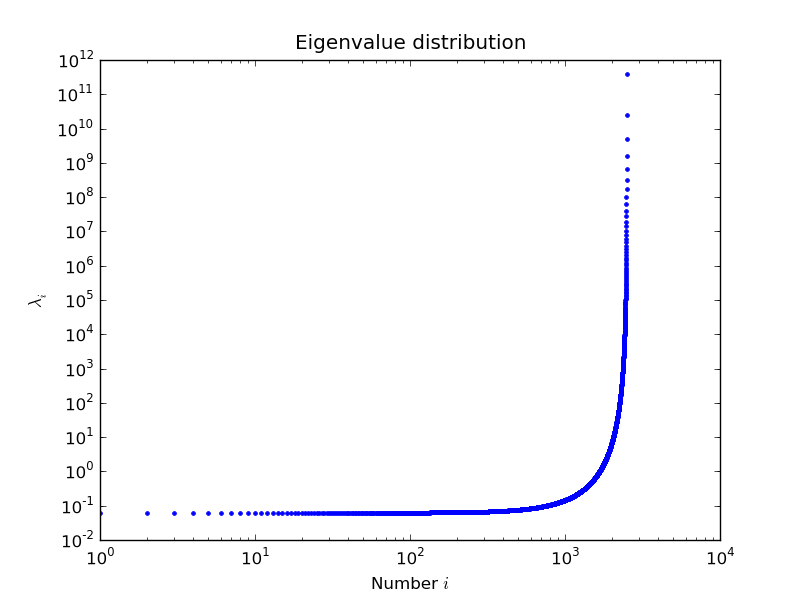
Another example by Nils Wagner:
Output:
$ python examples/lobpcg_sakurai.py
Results by LOBPCG for n=2500

[ 0.06250083  0.06250028  0.06250007]

Exact eigenvalues

[ 0.06250005  0.0625002   0.06250044]

Elapsed time 7.01