scikit-image: image processing

Author: Emmanuelle Gouillart

import numpy as np
import scipy as sp
import matplotlib.pyplot as plt

scikit-image is a Python package dedicated to image processing, using NumPy arrays as image objects. This chapter describes how to use scikit-image for various image processing tasks, and how it relates to other scientific Python modules such as NumPy and SciPy.

See also

For basic image manipulation, such as image cropping or simple filtering, a large number of simple operations can be realized with NumPy and SciPy only. See Image manipulation and processing using NumPy and SciPy.

Note that you should be familiar with the content of the previous chapter before reading the current one, as basic operations such as masking and labeling are a prerequisite.

Introduction and concepts

Images are NumPy’s arrays np.ndarray

Table 13 Terms

Pixels	array values: a[2, 3]
Channels	array dimensions
Image encoding	dtype (np.uint8, np.uint16, np.float)
Filters	functions (numpy, skimage, scipy)

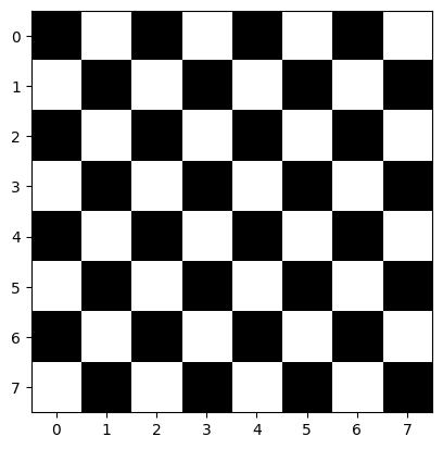
# This example shows how to create a simple checkerboard.
check = np.zeros((8, 8))
check[::2, 1::2] = 1
check[1::2, ::2] = 1
plt.imshow(check, cmap='gray', interpolation='nearest');

scikit-image and the scientific Python ecosystem

scikit-image is packaged in both pip and conda-based Python installations, as well as in most Linux distributions. Other Python packages for image processing & visualization that operate on NumPy arrays include:

Table 14 Other packages for working with images

scipy.ndimage	For N-dimensional arrays. Basic filtering, mathematical morphology, regions properties
Mahotas	With a focus on high-speed implementations.
Napari	A fast, interactive, multi-dimensional image viewer built in Qt.

Some powerful C++ image processing libraries also have Python bindings:

Table 15 C++ libraries with Python bindings

OpenCV	A highly optimized computer vision library with a focus on real-time applications.
ITK	The Insight ToolKit, especially useful for registration and working with 3D images.

To varying degrees, these C++-based libraries tend to be less Pythonic and NumPy-friendly.

What is included in scikit-image

• Website: https://scikit-image.org/

• Gallery of examples: https://scikit-image.org/docs/stable/auto_examples/

The library contains predominantly image processing algorithms, but also utility functions to ease data handling and processing. It contains the following submodules:

Table 16 Scikit-image submodules

skimage.color	Color space conversion.
skimage.data	Test images and example data.
skimage.draw	Drawing primitives (lines, text, etc.) that operate on NumPy arrays.
skimage.exposure	Image intensity adjustment, e.g., histogram equalization, etc.
skimage.feature	Feature detection and extraction, e.g., texture analysis corners, etc.
skimage.filters	Sharpening, edge finding, rank filters, thresholding, etc.
skimage.graph	Graph-theoretic operations, e.g., shortest paths.
skimage.io	Reading, saving, and displaying images and video.
skimage.measure	Measurement of image properties, e.g., region properties and contours.
skimage.metrics	Metrics corresponding to images, e.g. distance metrics, similarity, etc.
skimage.morphology	Morphological operations, e.g., opening or skeletonization.
skimage.restoration	Restoration algorithms, e.g., deconvolution algorithms, denoising, etc.
skimage.segmentation	Partitioning an image into multiple regions.
skimage.transform	Geometric and other transforms, e.g., rotation or the Radon transform.
skimage.util	Generic utilities.

Importing

We import scikit-image using the convention:

import skimage as ski

Most functionality lives in subpackages, e.g.:

image = ski.data.cat()

You can list all submodules with:

for m in dir(ski): print(m)

__version__
color
data
draw
exposure
feature
filters
future
graph
io
measure
metrics
morphology
registration
restoration
segmentation
transform
util

Most scikit-image functions take NumPy ndarrays as arguments

camera = ski.data.camera()
camera.dtype

dtype('uint8')

camera.shape

(512, 512)

filtered_camera = ski.filters.gaussian(camera, sigma=1)
type(filtered_camera)

numpy.ndarray

Example data

To start off, we need example images to work with. The library ships with a few of these:

skimage.data

image = ski.data.cat()
image.shape

(300, 451, 3)

Input/output, data types and colorspaces

I/O: skimage.io

Save an image to disk: skimage.io.imsave()

ski.io.imsave("cat.png", image)

Reading from files: skimage.io.imread()

cat = ski.io.imread("cat.png")

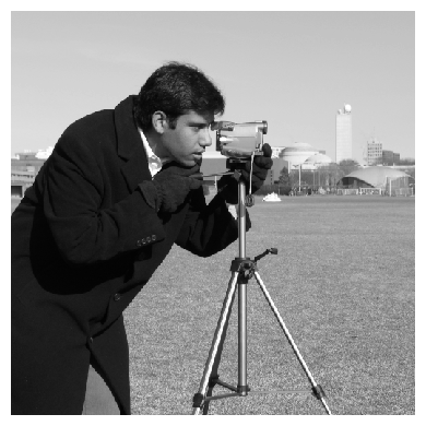
camera = ski.data.camera()

plt.figure(figsize=(4, 4))
plt.imshow(camera, cmap="gray", interpolation="nearest")
plt.axis("off")

plt.tight_layout()

This works with many data formats supported by the ImageIO library.

Loading also works with URLs:

logo = ski.io.imread('https://scikit-image.org/_static/img/logo.png')

Data types

Image ndarrays can be represented either by integers (signed or unsigned) or floats.

Careful with overflows with integer data types

camera = ski.data.camera()
camera.dtype
camera_multiply = 3 * camera

Show code cell source

Hide code cell source

plt.figure(figsize=(8, 4))
plt.subplot(121)
plt.imshow(camera, cmap="gray", interpolation="nearest")
plt.axis("off")
plt.subplot(122)
plt.imshow(camera_multiply, cmap="gray", interpolation="nearest")
plt.axis("off")

plt.tight_layout()

Different integer sizes are possible: 8-, 16- or 32-bytes, signed or unsigned.

Warning: An important (if questionable) skimage convention: float images are supposed to lie in [-1, 1] (in order to have comparable contrast for all float images):

camera_float = ski.util.img_as_float(camera)
camera.max(), camera_float.max()

(np.uint8(255), np.float64(1.0))

Some image processing routines need to work with float arrays, and may hence output an array with a different type and the data range from the input array

camera_sobel = ski.filters.sobel(camera)
camera_sobel.max()

np.float64(0.6447887988758096)

Utility functions are provided in skimage to convert both the dtype and the data range, following skimage’s conventions: util.img_as_float, util.img_as_ubyte, etc.

See the user guide for more details.

Colorspaces

Color images are of shape (N, M, 3) or (N, M, 4) (when an alpha channel encodes transparency)

face = sp.datasets.face()
face.shape

(768, 1024, 3)

Routines converting between different colorspaces (RGB, HSV, LAB etc.) are available in skimage.color : color.rgb2hsv, color.lab2rgb, etc. Check the docstring for the expected dtype (and data range) of input images.

3D images

Most functions of skimage can take 3D images as input arguments. Check the docstring to know if a function can be used on 3D images (for example MRI or CT images).

Exercise 68

Open a color image on your disk as a NumPy array.

Find a skimage function computing the histogram of an image and plot the histogram of each color channel

Convert the image to grayscale and plot its histogram.

Image preprocessing / enhancement

Goals: denoising, feature (edges) extraction, …

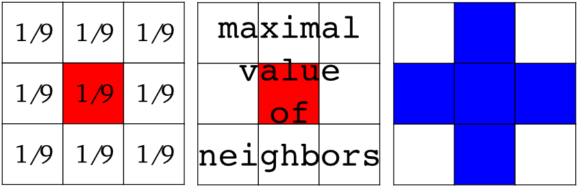
Local filters

Local filters replace the value of pixels by a function of the values of neighboring pixels. The function can be linear or non-linear.

Neighbourhood: square (choose size), disk, or more complicated structuring element.

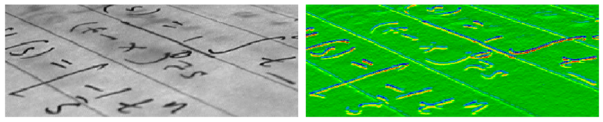
Example : horizontal Sobel filter

text = ski.data.text()
hsobel_text = ski.filters.sobel_h(text)

Uses the following linear kernel for computing horizontal gradients:

 1   2   1
 0   0   0
-1  -2  -1

Show code cell source

Hide code cell source

plt.figure(figsize=(12, 3))

plt.subplot(121)
plt.imshow(text, cmap="gray", interpolation="nearest")
plt.axis("off")
plt.subplot(122)
plt.imshow(hsobel_text, cmap="nipy_spectral", interpolation="nearest")
plt.axis("off")
plt.tight_layout()

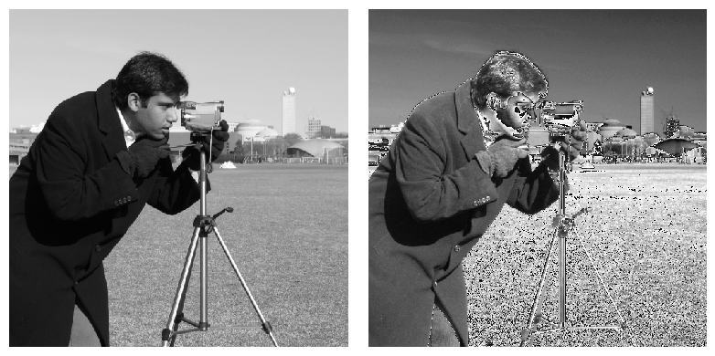
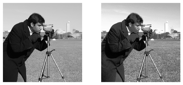
Non-local filters

Non-local filters use a large region of the image (or all the image) to transform the value of one pixel:

camera = ski.data.camera()
camera_equalized = ski.exposure.equalize_hist(camera)

Enhances contrast in large almost uniform regions.

Show code cell source

Hide code cell source

plt.figure(figsize=(7, 3))

plt.subplot(121)
plt.imshow(camera, cmap="gray", interpolation="nearest")
plt.axis("off")
plt.subplot(122)
plt.imshow(camera_equalized, cmap="gray", interpolation="nearest")
plt.axis("off")
plt.tight_layout()

Mathematical morphology

See wikipedia for an introduction on mathematical morphology.

Probe an image with a simple shape (a structuring element), and modify this image according to how the shape locally fits or misses the image.

Default structuring element: 4-connectivity of a pixel

# Import structuring elements to make them more easily accessible
from skimage.morphology import disk, diamond

diamond(1)

array([[0, 1, 0],
       [1, 1, 1],
       [0, 1, 0]], dtype=uint8)

Erosion = minimum filter. Replace the value of a pixel by the minimal value covered by the structuring element.:

a = np.zeros((7,7), dtype=np.uint8)
a[1:6, 2:5] = 1
a

array([[0, 0, 0, 0, 0, 0, 0],
       [0, 0, 1, 1, 1, 0, 0],
       [0, 0, 1, 1, 1, 0, 0],
       [0, 0, 1, 1, 1, 0, 0],
       [0, 0, 1, 1, 1, 0, 0],
       [0, 0, 1, 1, 1, 0, 0],
       [0, 0, 0, 0, 0, 0, 0]], dtype=uint8)

ski.morphology.binary_erosion(a, diamond(1)).astype(np.uint8)

array([[0, 0, 0, 0, 0, 0, 0],
       [0, 0, 0, 0, 0, 0, 0],
       [0, 0, 0, 1, 0, 0, 0],
       [0, 0, 0, 1, 0, 0, 0],
       [0, 0, 0, 1, 0, 0, 0],
       [0, 0, 0, 0, 0, 0, 0],
       [0, 0, 0, 0, 0, 0, 0]], dtype=uint8)

#Erosion removes objects smaller than the structure
ski.morphology.binary_erosion(a, diamond(2)).astype(np.uint8)

array([[0, 0, 0, 0, 0, 0, 0],
       [0, 0, 0, 0, 0, 0, 0],
       [0, 0, 0, 0, 0, 0, 0],
       [0, 0, 0, 0, 0, 0, 0],
       [0, 0, 0, 0, 0, 0, 0],
       [0, 0, 0, 0, 0, 0, 0],
       [0, 0, 0, 0, 0, 0, 0]], dtype=uint8)

Dilation: maximum filter:

a = np.zeros((5, 5))
a[2, 2] = 1
a

array([[0., 0., 0., 0., 0.],
       [0., 0., 0., 0., 0.],
       [0., 0., 1., 0., 0.],
       [0., 0., 0., 0., 0.],
       [0., 0., 0., 0., 0.]])

ski.morphology.binary_dilation(a, diamond(1)).astype(np.uint8)

array([[0, 0, 0, 0, 0],
       [0, 0, 1, 0, 0],
       [0, 1, 1, 1, 0],
       [0, 0, 1, 0, 0],
       [0, 0, 0, 0, 0]], dtype=uint8)

Opening: erosion + dilation:

a = np.zeros((5,5), dtype=int)
a[1:4, 1:4] = 1; a[4, 4] = 1
a

array([[0, 0, 0, 0, 0],
       [0, 1, 1, 1, 0],
       [0, 1, 1, 1, 0],
       [0, 1, 1, 1, 0],
       [0, 0, 0, 0, 1]])

ski.morphology.binary_opening(a, diamond(1)).astype(np.uint8)

array([[0, 0, 0, 0, 0],
       [0, 0, 1, 0, 0],
       [0, 1, 1, 1, 0],
       [0, 0, 1, 0, 0],
       [0, 0, 0, 0, 0]], dtype=uint8)

Opening removes small objects and smoothes corners.

Grayscale mathematical morphology

Mathematical morphology operations are also available for (non-binary) grayscale images (int or float type). Erosion and dilation correspond to minimum (resp. maximum) filters.

Higher-level mathematical morphology are available: tophat, skeletonization, etc.

See also

Basic mathematical morphology is also implemented in scipy.ndimage.morphology. The scipy.ndimage implementation works on arbitrary-dimensional arrays.

---

Example of filters comparison: image denoising

coins = ski.data.coins()
coins_zoom = coins[10:80, 300:370]
median_coins = ski.filters.median(
    coins_zoom, disk(1)
)
tv_coins = ski.restoration.denoise_tv_chambolle(
    coins_zoom, weight=0.1
)
gaussian_filter_coins = ski.filters.gaussian(coins, sigma=2)
med_filter_coins = ski.filters.median(coins, np.ones((3, 3)))
tv_filter_coins = ski.restoration.denoise_tv_chambolle(coins, weight=0.1)

Show code cell source

Hide code cell source

plt.figure(figsize=(16, 4))
plt.subplot(141)
plt.imshow(coins[10:80, 300:370], cmap="gray", interpolation="nearest")
plt.axis("off")
plt.title("Image")
plt.subplot(142)
plt.imshow(gaussian_filter_coins[10:80, 300:370], cmap="gray", interpolation="nearest")
plt.axis("off")
plt.title("Gaussian filter")
plt.subplot(143)
plt.imshow(med_filter_coins[10:80, 300:370], cmap="gray", interpolation="nearest")
plt.axis("off")
plt.title("Median filter")
plt.subplot(144)
plt.imshow(tv_filter_coins[10:80, 300:370], cmap="gray", interpolation="nearest")
plt.axis("off")
plt.title("TV filter")

Text(0.5, 1.0, 'TV filter')

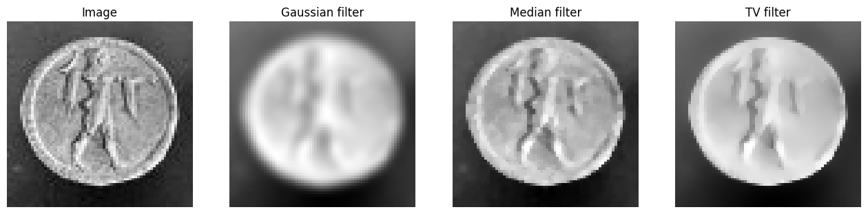
Image segmentation

Image segmentation is the attribution of different labels to different regions of the image, for example in order to extract the pixels of an object of interest.

Binary segmentation: foreground + background

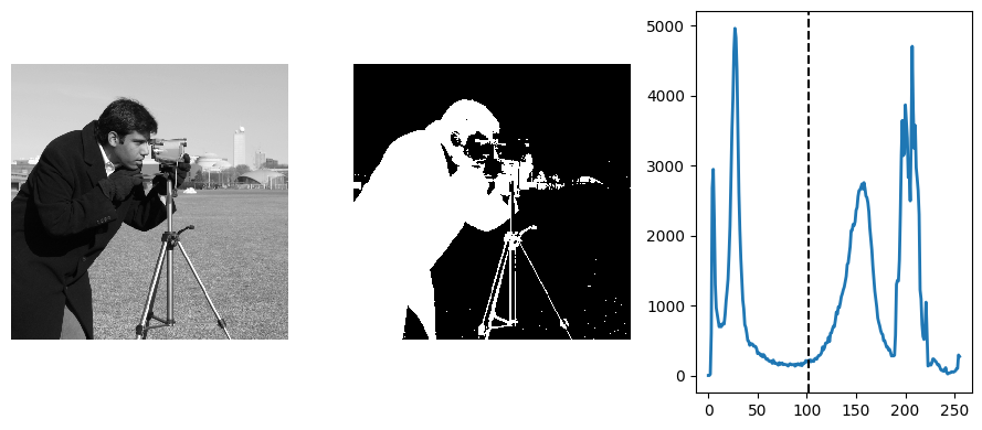
Histogram-based method: Otsu thresholding

Note

The Otsu method is a simple heuristic to find a threshold to separate the foreground from the background.

Earlier scikit-image versions

skimage.filters is called skimage.filter in earlier versions of scikit-image

camera = ski.data.camera()
val = ski.filters.threshold_otsu(camera)
mask = camera < val

# The histogram from which Otsu calculated the threshold.
hist, bins_center = ski.exposure.histogram(camera)

Show code cell source

Hide code cell source

plt.figure(figsize=(9, 4))
plt.subplot(131)
plt.imshow(camera, cmap="gray", interpolation="nearest")
plt.axis("off")
plt.subplot(132)
plt.imshow(mask, cmap="gray", interpolation="nearest")
plt.axis("off")
plt.subplot(133)
plt.plot(bins_center, hist, lw=2)
plt.axvline(val, color="k", ls="--")

plt.tight_layout()

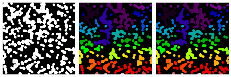
Labeling connected components of a discrete image

Note

Once you have separated foreground objects, it is use to separate them from each other. For this, we can assign a different integer labels to each one.

Synthetic data:

n = 20
l = 256
im = np.zeros((l, l))
rng = np.random.default_rng()
points = l * rng.random((2, n ** 2))
im[(points[0]).astype(int), (points[1]).astype(int)] = 1
im = ski.filters.gaussian(im, sigma=l / (4. * n))
blobs = im > im.mean()

Label all connected components:

all_labels = ski.measure.label(blobs)

Label only foreground connected components:

blobs_labels = ski.measure.label(blobs, background=0)

Show code cell source

Hide code cell source

plt.figure(figsize=(9, 3.5))
plt.subplot(131)
plt.imshow(blobs, cmap="gray")
plt.axis("off")
plt.subplot(132)
plt.imshow(all_labels, cmap="nipy_spectral")
plt.axis("off")
plt.subplot(133)
plt.imshow(blobs_labels, cmap="nipy_spectral")
plt.axis("off")

plt.tight_layout()

See also

scipy.ndimage.find_objects() is useful to return slices on object in an image.

Marker based methods

If you have markers inside a set of regions, you can use these to segment the regions.

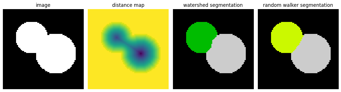
Watershed segmentation

The Watershed (skimage.segmentation.watershed()) is a region-growing approach that fills “basins” in the image

# Generate an initial image with two overlapping circles
x, y = np.indices((80, 80))
x1, y1, x2, y2 = 28, 28, 44, 52
r1, r2 = 16, 20
mask_circle1 = (x - x1) ** 2 + (y - y1) ** 2 < r1 ** 2
mask_circle2 = (x - x2) ** 2 + (y - y2) ** 2 < r2 ** 2
image = np.logical_or(mask_circle1, mask_circle2)
# Now we want to separate the two objects in image
# Generate the markers as local maxima of the distance
# to the background
# Use scipy.ndimage.distance_transform_edt
distance = sp.ndimage.distance_transform_edt(image)
peak_idx = ski.feature.peak_local_max(
    distance, footprint=np.ones((3, 3)), labels=image
)
peak_mask = np.zeros_like(distance, dtype=bool)
peak_mask[tuple(peak_idx.T)] = True
markers = ski.morphology.label(peak_mask)
labels_ws = ski.segmentation.watershed(
    -distance, markers, mask=image
)

Random walker segmentation

The random walker algorithm (skimage.segmentation.random_walker()) is similar to the Watershed, but with a more “probabilistic” approach. It is based on the idea of the diffusion of labels in the image:

# Transform markers image so that 0-valued pixels are to
# be labelled, and -1-valued pixels represent background
markers[~image] = -1
labels_rw = ski.segmentation.random_walker(image, markers)

Show code cell source

Hide code cell source

plt.figure(figsize=(12, 3.5))
plt.subplot(141)
plt.imshow(image, cmap="gray", interpolation="nearest")
plt.axis("off")
plt.title("image")
plt.subplot(142)
plt.imshow(-distance, interpolation="nearest")
plt.axis("off")
plt.title("distance map")
plt.subplot(143)
plt.imshow(labels_ws, cmap="nipy_spectral", interpolation="nearest")
plt.axis("off")
plt.title("watershed segmentation")
plt.subplot(144)
plt.imshow(labels_rw, cmap="nipy_spectral", interpolation="nearest")
plt.axis("off")
plt.title("random walker segmentation")

plt.tight_layout()

Postprocessing label images

skimage provides several utility functions that can be used on label images (ie images where different discrete values identify different regions). Functions names are often self-explaining: skimage.segmentation.clear_border(), skimage.segmentation.relabel_from_one(), skimage.morphology.remove_small_objects(), etc.

Exercise 69

• Load the coins image from the data submodule.

• Separate the coins from the background by testing several segmentation methods: Otsu thresholding, adaptive thresholding, and watershed or random walker segmentation.

• If necessary, use a postprocessing function to improve the coins / background segmentation.

Measuring regions’ properties

Example: compute the size and perimeter of the two segmented regions:

properties = ski.measure.regionprops(labels_rw)
[float(prop.area) for prop in properties]

[770.0, 1168.0]

[prop.perimeter for prop in properties]

[np.float64(100.91168824543142), np.float64(126.81118318204308)]

See also

for some properties, functions are available as well in scipy.ndimage.measurements with a different API (a list is returned).

Exercise 70

• Use the binary image of the coins and background from the previous exercise.

• Compute an image of labels for the different coins.

• Compute the size and eccentricity of all coins.

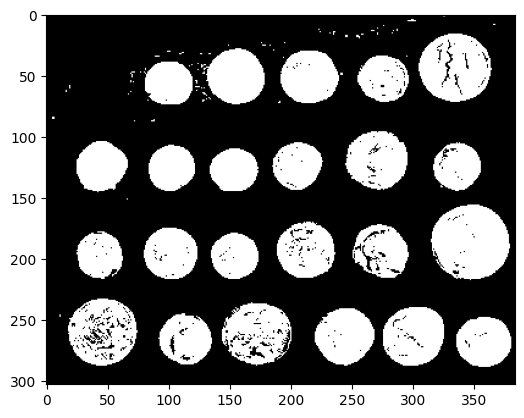
Data visualization and interaction

Meaningful visualizations are useful when testing a given processing pipeline.

Some image processing operations:

coins = ski.data.coins()
mask = coins > ski.filters.threshold_otsu(coins)
clean_border = ski.segmentation.clear_border(mask)

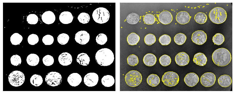
Visualize binary result:

plt.figure()
plt.imshow(clean_border, cmap='gray')

<matplotlib.image.AxesImage at 0x1119770e0>

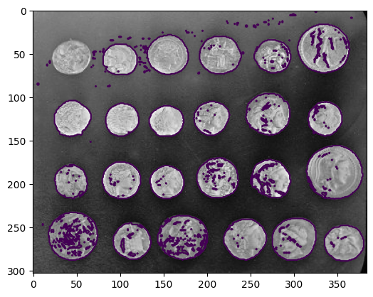
Visualize contour

plt.figure()
plt.imshow(coins, cmap='gray')
plt.contour(clean_border, [0.5])

<matplotlib.contour.QuadContourSet at 0x111e45b20>

Use skimage dedicated utility function:

coins_edges = ski.segmentation.mark_boundaries(
    coins, clean_border.astype(int)
)

Show code cell source

Hide code cell source

plt.figure(figsize=(8, 3.5))
plt.subplot(121)
plt.imshow(clean_border, cmap="gray")
plt.axis("off")
plt.subplot(122)
plt.imshow(coins_edges)
plt.axis("off")

plt.tight_layout()

Feature extraction for computer vision

Geometric or textural descriptor can be extracted from images in order to

• classify parts of the image (e.g. sky vs. buildings)

• match parts of different images (e.g. for object detection)

• and many other applications of Computer Vision

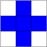
Example: detecting corners using Harris detector

tform = ski.transform.AffineTransform(
    scale=(1.3, 1.1), rotation=1, shear=0.7,
    translation=(210, 50)
)

image = ski.transform.warp(
    ski.data.checkerboard(), tform.inverse, output_shape=(350, 350)
)

coords = ski.feature.corner_peaks(
    ski.feature.corner_harris(image), min_distance=5
)
coords_subpix = ski.feature.corner_subpix(
    image, coords, window_size=13
)

Show code cell source

Hide code cell source

plt.gray()
plt.imshow(image, interpolation="nearest")
plt.plot(coords_subpix[:, 1], coords_subpix[:, 0], "+r", markersize=15, mew=5)
plt.plot(coords[:, 1], coords[:, 0], ".b", markersize=7)
plt.axis("off")

(np.float64(-23.504322001100714),
 np.float64(349.5),
 np.float64(349.5),
 np.float64(-0.5))

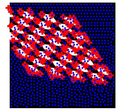
(this example is taken from the plot_corner example in scikit-image)

Points of interest such as corners can then be used to match objects in different images, as described in the plot_matching example of scikit-image.