sympy : Symbolic Mathematics in Python

Author: Fabian Pedregosa

Objectives

1. Evaluate expressions with arbitrary precision.

2. Perform algebraic manipulations on symbolic expressions.

3. Perform basic calculus tasks (limits, differentiation and : integration) with symbolic expressions.

4. Solve polynomial and transcendental equations.

5. Solve some differential equations.

What is SymPy? SymPy is a Python library for symbolic mathematics. It aims to be an alternative to systems such as Mathematica or Maple while keeping the code as simple as possible and easily extensible. SymPy is written entirely in Python and does not require any external libraries.

Sympy documentation and packages for installation can be found on https://www.sympy.org/

First Steps with SymPy

Using SymPy as a calculator

SymPy defines three numerical types: Real, Rational and Integer.

The Rational class represents a rational number as a pair of two Integers: the numerator and the denominator, so Rational(1, 2) represents 1/2, Rational(5, 2) 5/2 and so on:

import sympy as sym
a = sym.Rational(1, 2)

a

\[\displaystyle \frac{1}{2}\]

a*2

\[\displaystyle 1\]

SymPy uses mpmath in the background, which makes it possible to perform computations using arbitrary-precision arithmetic. That way, some special constants, like \(e\), \(pi\), \(oo\) (Infinity), are treated as symbols and can be evaluated with arbitrary precision:

sym.pi**2

\[\displaystyle \pi^{2}\]

sym.pi.evalf()

\[\displaystyle 3.14159265358979\]

(sym.pi + sym.exp(1)).evalf()

\[\displaystyle 5.85987448204884\]

as you see, evalf evaluates the expression to a floating-point number.

There is also a class representing mathematical infinity, called oo:

sym.oo > 99999

\[\displaystyle \text{True}\]

sym.oo + 1

\[\displaystyle \infty\]

Exercise 63

1. Calculate \(\sqrt{2}\) with 100 decimals.

2. Calculate \(1/2 + 1/3\) in rational arithmetic.

Symbols

In contrast to other Computer Algebra Systems, in SymPy you have to declare symbolic variables explicitly:

x = sym.Symbol('x')
y = sym.Symbol('y')

Then you can manipulate them:

x + y + x - y

\[\displaystyle 2 x\]

(x + y) ** 2

\[\displaystyle \left(x + y\right)^{2}\]

Symbols can now be manipulated using some of python operators: +, -, *, ** (arithmetic), &, |, ~, >>, << (boolean).

Printing

Sympy allows for control of the display of the output. From here we use the following setting for printing:

sym.init_printing(use_unicode=False, wrap_line=True)

Algebraic manipulations

SymPy is capable of performing powerful algebraic manipulations. We’ll take a look into some of the most frequently used: expand and simplify.

Expand

Use this to expand an algebraic expression. It will try to denest powers and multiplications:

sym.expand((x + y) ** 3)

3 * x * y ** 2 + 3 * y * x ** 2 + x ** 3 + y ** 3

Further options can be given in form on keywords:

sym.expand(x + y, complex=True)

sym.I * sym.im(x) + sym.I * sym.im(y) + sym.re(x) + sym.re(y)

sym.expand(sym.cos(x + y), trig=True)

sym.cos(x) * sym.cos(y) - sym.sin(x) * sym.sin(y)

Simplify

Use simplify if you would like to transform an expression into a simpler form:

sym.simplify((x + x * y) / x)

Simplification is a somewhat vague term, and more precises alternatives to simplify exists: powsimp (simplification of exponents), trigsimp (for trigonometric expressions) , logcombine, radsimp, together.

Exercise 64

1. Calculate the expanded form of \((x+y)^6\).

2. Simplify the trigonometric expression \(\sin(x) / \cos(x)\)

Calculus

Limits

Limits are easy to use in SymPy, they follow the syntax limit(function, variable, point), so to compute the limit of \(f(x)\) as \(x \rightarrow 0\), you would issue limit(f, x, 0):

sym.limit(sym.sin(x) / x, x, 0)

you can also calculate the limit at infinity:

sym.limit(x, x, sym.oo)

sym.limit(1 / x, x, sym.oo)

sym.limit(x ** x, x, 0)

Differentiation

You can differentiate any SymPy expression using diff(func, var). Examples:

sym.diff(sym.sin(x), x)

sym.diff(sym.sin(2 * x), x)

sym.diff(sym.tan(x), x)

You can check that it is correct by:

sym.limit((sym.tan(x + y) - sym.tan(x)) / y, y, 0)

Which is equivalent since

\[ \sec(x) = \frac{1}{\cos(x)} and \sec^2(x) = \tan^2(x) + 1. \]

You can check this as well:

sym.trigsimp(sym.diff(sym.tan(x), x))

Higher derivatives can be calculated using the diff(func, var, n) method:

sym.diff(sym.sin(2 * x), x, 1)

sym.diff(sym.sin(2 * x), x, 2)

sym.diff(sym.sin(2 * x), x, 3)

Series expansion

SymPy also knows how to compute the Taylor series of an expression at a point. Use series(expr, var):

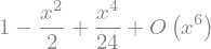
sym.series(sym.cos(x), x)

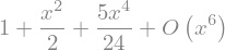
sym.series(1/sym.cos(x), x)

Exercise 65

1. Calculate \(\lim_{x\rightarrow 0} \sin(x)/x\)

2. Calculate the derivative of \(log(x)\) for \(x\).

Integration

SymPy has support for indefinite and definite integration of transcendental elementary and special functions via integrate() facility, which uses the powerful extended Risch-Norman algorithm and some heuristics and pattern matching. You can integrate elementary functions:

sym.integrate(6 * x ** 5, x)

sym.integrate(sym.sin(x), x)

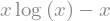
sym.integrate(sym.log(x), x)

sym.integrate(2 * x + sym.sinh(x), x)

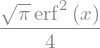
Also special functions are handled easily:

sym.integrate(sym.exp(-x ** 2) * sym.erf(x), x)

It is possible to compute definite integral:

sym.integrate(x**3, (x, -1, 1))

sym.integrate(sym.sin(x), (x, 0, sym.pi / 2))

sym.integrate(sym.cos(x), (x, -sym.pi / 2, sym.pi / 2))

Also improper integrals are supported as well:

sym.integrate(sym.exp(-x), (x, 0, sym.oo))

sym.integrate(sym.exp(-x ** 2), (x, -sym.oo, sym.oo))

Equation solving

SymPy is able to solve algebraic equations, in one and several variables using solveset():

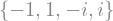
sym.solveset(x ** 4 - 1, x)

As you can see it takes as first argument an expression that is supposed to be equaled to 0. It also has (limited) support for transcendental equations:

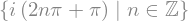
sym.solveset(sym.exp(x) + 1, x)

Systems of linear equations

Sympy is able to solve a large part of polynomial equations, and is also capable of solving multiple equations with respect to multiple variables giving a tuple as second argument. To do this you use the solve() command:

solution = sym.solve((x + 5 * y - 2, -3 * x + 6 * y - 15), (x, y))
solution[x], solution[y]

Another alternative in the case of polynomial equations is factor. factor returns the polynomial factorized into irreducible terms, and is capable of computing the factorization over various domains:

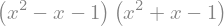
f = x ** 4 - 3 * x ** 2 + 1
sym.factor(f)

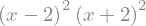
sym.factor(f, modulus=5)

SymPy is also able to solve boolean equations, that is, to decide if a certain boolean expression is satisfiable or not. For this, we use the function satisfiable:

sym.satisfiable(x & y)

{y: True, x: True}

This tells us that (x & y) is True whenever x and y are both True. If an expression cannot be true, i.e. no values of its arguments can make the expression True, it will return False:

sym.satisfiable(x & ~x)

False

Exercise 66

1. Solve the system of equations \(x + y = 2\), \(2\cdot x + y = 0\)

2. Are there boolean values x, y that make (~x | y) & (~y | x) true?

Linear Algebra

Matrices

Matrices are created as instances from the Matrix class:

sym.Matrix([[1, 0], [0, 1]])

unlike a NumPy array, you can also put Symbols in it:

x, y = sym.symbols('x, y')
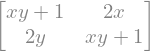
A = sym.Matrix([[1, x], [y, 1]])
A

A**2

Differential Equations

SymPy is capable of solving (some) Ordinary Differential. To solve differential equations, use dsolve. First, create an undefined function by passing cls=Function to the symbols function:

f, g = sym.symbols('f g', cls=sym.Function)

f and g are now undefined functions. We can call f(x), and it will represent an unknown function:

f(x)

f(x).diff(x, x) + f(x)

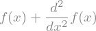
sym.dsolve(f(x).diff(x, x) + f(x), f(x))

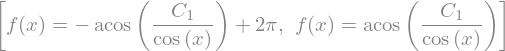
Keyword arguments can be given to this function in order to help if find the best possible resolution system. For example, if you know that it is a separable equations, you can use keyword hint='separable' to force dsolve to resolve it as a separable equation:

sym.dsolve(sym.sin(x) * sym.cos(f(x)) + sym.cos(x) * sym.sin(f(x)) * f(x).diff(x), f(x), hint='separable')

Exercise 67

1. Solve the Bernoulli differential equation

   \[ x \frac{d f(x)}{x} + f(x) - f(x)^2=0 \]

2. Solve the same equation using hint='Bernoulli'. What do you observe ?