Statistics in Python

Author: Gaël Varoquaux

Requirements

• Standard scientific Python environment (NumPy, SciPy, matplotlib)

• Pandas

• Statsmodels

• Seaborn

To install Python and these dependencies, we recommend that you download Anaconda Python or, preferably, use the package manager if you are under Ubuntu or other linux.

See also

• Bayesian statistics in Python: This chapter does not cover tools for Bayesian statistics. Of particular interest for Bayesian modelling is PyMC, which implements a probabilistic programming language in Python.

• Read a statistics book: The Think stats book is available as free PDF or in print and is a great introduction to statistics.

import numpy as np
import matplotlib.pyplot as plt
import pandas as pd

Note

Why Python for statistics?

R is a language dedicated to statistics. Python is a general-purpose language with statistics modules. R has more statistical analysis features than Python, and specialized syntaxes. However, when it comes to building complex analysis pipelines that mix statistics with e.g. image analysis, text mining, or control of a physical experiment, the richness of Python is an invaluable asset.

Note

In this document, the Python inputs are represented with the sign “>>>”.

Disclaimer: Gender questions

Some of the examples of this tutorial are chosen around gender questions. The reason is that on such questions controlling the truth of a claim actually matters to many people.

Data representation and interaction

Data as a table

The setting that we consider for statistical analysis is that of multiple observations or samples described by a set of different attributes or features. The data can than be seen as a 2D table, or matrix, with columns giving the different attributes of the data, and rows the observations. For instance, the data contained in examples/brain_size.csv:

"";"Gender";"FSIQ";"VIQ";"PIQ";"Weight";"Height";"MRI_Count"
"1";"Female";133;132;124;"118";"64.5";816932
"2";"Male";140;150;124;".";"72.5";1001121
"3";"Male";139;123;150;"143";"73.3";1038437
"4";"Male";133;129;128;"172";"68.8";965353
"5";"Female";137;132;134;"147";"65.0";951545

The pandas data-frame

Note

We will store and manipulate this data in a pandas.DataFrame, from the pandas module. It is the Python equivalent of the spreadsheet table. It is different from a 2D numpy array as it has named columns, can contain a mixture of different data types by column, and has elaborate selection and pivotal mechanisms.

Creating dataframes: reading data files or converting arrays

Separator

It is a CSV file, but the separator is “;”

Reading from a CSV file: Using the above CSV file that gives observations of brain size and weight and IQ (Willerman et al. 1991), the data are a mixture of numerical and categorical values:

data = pd.read_csv('examples/brain_size.csv', sep=';', na_values=".", index_col=0)
data

	Gender	FSIQ	VIQ	PIQ	Weight	Height	MRI_Count
1	Female	133	132	124	118.0	64.5	816932
2	Male	140	150	124	NaN	72.5	1001121
3	Male	139	123	150	143.0	73.3	1038437
4	Male	133	129	128	172.0	68.8	965353
5	Female	137	132	134	147.0	65.0	951545
6	Female	99	90	110	146.0	69.0	928799
7	Female	138	136	131	138.0	64.5	991305
8	Female	92	90	98	175.0	66.0	854258
9	Male	89	93	84	134.0	66.3	904858
10	Male	133	114	147	172.0	68.8	955466
11	Female	132	129	124	118.0	64.5	833868
12	Male	141	150	128	151.0	70.0	1079549
13	Male	135	129	124	155.0	69.0	924059
14	Female	140	120	147	155.0	70.5	856472
15	Female	96	100	90	146.0	66.0	878897
16	Female	83	71	96	135.0	68.0	865363
17	Female	132	132	120	127.0	68.5	852244
18	Male	100	96	102	178.0	73.5	945088
19	Female	101	112	84	136.0	66.3	808020
20	Male	80	77	86	180.0	70.0	889083
21	Male	83	83	86	NaN	NaN	892420
22	Male	97	107	84	186.0	76.5	905940
23	Female	135	129	134	122.0	62.0	790619
24	Male	139	145	128	132.0	68.0	955003
25	Female	91	86	102	114.0	63.0	831772
26	Male	141	145	131	171.0	72.0	935494
27	Female	85	90	84	140.0	68.0	798612
28	Male	103	96	110	187.0	77.0	1062462
29	Female	77	83	72	106.0	63.0	793549
30	Female	130	126	124	159.0	66.5	866662
31	Female	133	126	132	127.0	62.5	857782
32	Male	144	145	137	191.0	67.0	949589
33	Male	103	96	110	192.0	75.5	997925
34	Male	90	96	86	181.0	69.0	879987
35	Female	83	90	81	143.0	66.5	834344
36	Female	133	129	128	153.0	66.5	948066
37	Male	140	150	124	144.0	70.5	949395
38	Female	88	86	94	139.0	64.5	893983
39	Male	81	90	74	148.0	74.0	930016
40	Male	89	91	89	179.0	75.5	935863

Warning

Missing values

The weight of the second individual is missing in the CSV file. If we don’t specify the missing value (NA = not available) marker, we will not be able to do statistical analysis.

Creating from arrays: A pandas.DataFrame can also be seen as a dictionary of 1D ‘series’, eg arrays or lists. If we have 3 numpy arrays:

t = np.linspace(-6, 6, 20)
sin_t = np.sin(t)
cos_t = np.cos(t)

We can expose them as a pd.DataFrame

pd.DataFrame({'t': t, 'sin': sin_t, 'cos': cos_t})

	t	sin	cos
0	-6.000000	0.279415	0.960170
1	-5.368421	0.792419	0.609977
2	-4.736842	0.999701	0.024451
3	-4.105263	0.821291	-0.570509
4	-3.473684	0.326021	-0.945363
5	-2.842105	-0.295030	-0.955488
6	-2.210526	-0.802257	-0.596979
7	-1.578947	-0.999967	-0.008151
8	-0.947368	-0.811882	0.583822
9	-0.315789	-0.310567	0.950551
10	0.315789	0.310567	0.950551
11	0.947368	0.811882	0.583822
12	1.578947	0.999967	-0.008151
13	2.210526	0.802257	-0.596979
14	2.842105	0.295030	-0.955488
15	3.473684	-0.326021	-0.945363
16	4.105263	-0.821291	-0.570509
17	4.736842	-0.999701	0.024451
18	5.368421	-0.792419	0.609977
19	6.000000	-0.279415	0.960170

Other inputs: pandas can input data from SQL, excel files, or other formats. See the pandas documentation.

Manipulating data

data is a pandas.DataFrame, that resembles R’s dataframe:

data.shape    # 40 rows and 8 columns

(40, 7)

data.columns  # It has columns

Index(['Gender', 'FSIQ', 'VIQ', 'PIQ', 'Weight', 'Height', 'MRI_Count'], dtype='object')

data['Gender']  # Columns can be addressed by name

1     Female
2       Male
3       Male
4       Male
5     Female
6     Female
7     Female
8     Female
9       Male
10      Male
11    Female
12      Male
13      Male
14    Female
15    Female
16    Female
17    Female
18      Male
19    Female
20      Male
21      Male
22      Male
23    Female
24      Male
25    Female
26      Male
27    Female
28      Male
29    Female
30    Female
31    Female
32      Male
33      Male
34      Male
35    Female
36    Female
37      Male
38    Female
39      Male
40      Male
Name: Gender, dtype: object

# Simpler selector
data[data['Gender'] == 'Female']['VIQ'].mean()

np.float64(109.45)

Note

For a quick view on a large dataframe, use its describe method: pandas.DataFrame.describe().

groupby: splitting a dataframe on values of categorical variables:

groupby_gender = data.groupby('Gender')
for gender, value in groupby_gender['VIQ']:
    print((gender, value.mean()))

('Female', np.float64(109.45))
('Male', np.float64(115.25))

groupby_gender is a powerful object that exposes many operations on the resulting group of dataframes:

groupby_gender.mean()

	FSIQ	VIQ	PIQ	Weight	Height	MRI_Count
Gender
Female	111.9	109.45	110.45	137.200000	65.765000	862654.6
Male	115.0	115.25	111.60	166.444444	71.431579	954855.4

Note

Use tab-completion on groupby_gender to find more. Other common grouping functions are median, count (useful for checking to see the amount of missing values in different subsets) or sum. Groupby evaluation is lazy, no work is done until an aggregation function is applied.

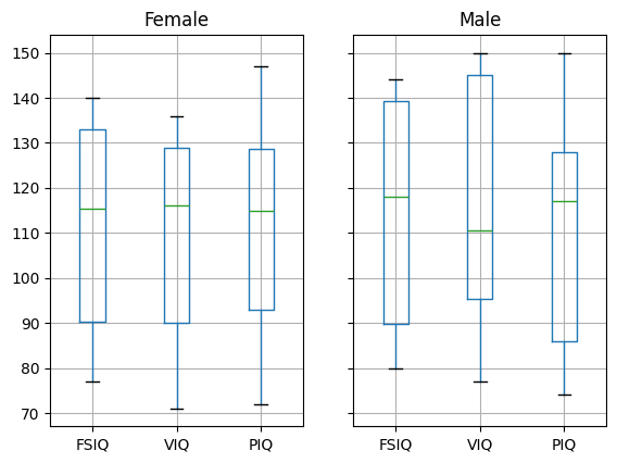
data = pd.read_csv("examples/brain_size.csv", sep=";", na_values=".")

# Box plots of different columns for each gender
groupby_gender = data.groupby("Gender")
groupby_gender.boxplot(column=["FSIQ", "VIQ", "PIQ"]);

Exercise 58

• What is the mean value for VIQ for the full population?

• How many males/females were included in this study?

  Hint use ‘tab completion’ to find out the methods that can be called, instead of ‘mean’ in the above example.

• What is the average value of MRI counts expressed in log units, for males and females?

Note

groupby_gender.boxplot is used for the plots above (see the plot code above).

Plotting data

Pandas comes with some plotting tools (pandas.plotting, using matplotlib behind the scene) to display statistics of the data in dataframes:

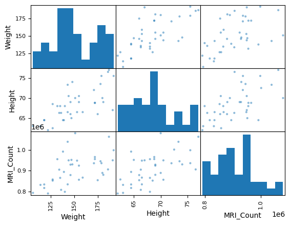
Scatter matrices:

pd.plotting.scatter_matrix(data[['Weight', 'Height', 'MRI_Count']]);

Two populations

The IQ metrics are bimodal, as if there are 2 sub-populations.

pd.plotting.scatter_matrix(data[['PIQ', 'VIQ', 'FSIQ']]);

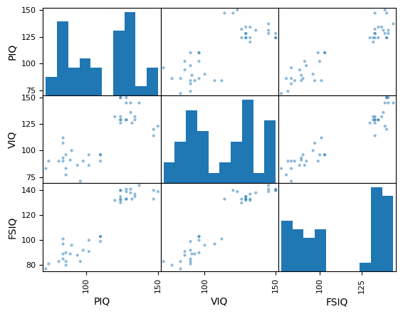
Exercise 59

Plot the scatter matrix for males only, and for females only. Do you think that the 2 sub-populations correspond to gender?

Hypothesis testing: comparing two groups

For simple statistical tests, we will use the scipy.stats sub-module of SciPy:

import scipy as sp

See also

SciPy is a vast library. For a quick summary to the whole library, see the scipy chapter.

Student’s t-test: the simplest statistical test

One-sample tests: testing the value of a population mean

scipy.stats.ttest_1samp() tests the null hypothesis that the mean of the population underlying the data is equal to a given value. It returns the T statistic, and the p-value (see the function’s help):

sp.stats.ttest_1samp(data['VIQ'], 0)

TtestResult(statistic=np.float64(30.08809997084933), pvalue=np.float64(1.3289196468727879e-28), df=np.int64(39))

The p-value of \(10^-28\) indicates that such an extreme value of the statistic is unlikely to be observed under the null hypothesis. This may be taken as evidence that the null hypothesis is false and that the population mean IQ (VIQ measure) is not 0.

Technically, the p-value of the t-test is derived under the assumption that the means of samples drawn from the population are normally distributed. This condition is exactly satisfied when the population itself is normally distributed; however, due to the central limit theorem, the condition is nearly true for reasonably large samples drawn from populations that follow a variety of non-normal distributions.

Nonetheless, if we are concerned that violation of the normality assumptions will affect the conclusions of the test, we can use a Wilcoxon signed-rank test, which relaxes this assumption at the expense of test power:

sp.stats.wilcoxon(data['VIQ'])

WilcoxonResult(statistic=np.float64(0.0), pvalue=np.float64(3.488172636231201e-08))

Two-sample t-test: testing for difference across populations

We have seen above that the mean VIQ in the male and female samples were different. To test whether this difference is significant (and suggests that there is a difference in population means), we perform a two-sample t-test using scipy.stats.ttest_ind():

female_viq = data[data['Gender'] == 'Female']['VIQ']
male_viq = data[data['Gender'] == 'Male']['VIQ']
sp.stats.ttest_ind(female_viq, male_viq)

TtestResult(statistic=np.float64(-0.7726161723275012), pvalue=np.float64(0.44452876778583217), df=np.float64(38.0))

The corresponding non-parametric test is the Mann–Whitney U test, scipy.stats.mannwhitneyu().

sp.stats.mannwhitneyu(female_viq, male_viq)

MannwhitneyuResult(statistic=np.float64(164.5), pvalue=np.float64(0.3422886868727315))

Paired tests: repeated measurements on the same individuals

# Box plot of FSIQ and PIQ (different measures of IQ)
plt.figure(figsize=(4, 3))
data.boxplot(column=["FSIQ", "PIQ"])

<Axes: >

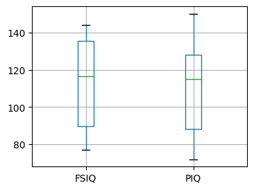
PIQ, VIQ, and FSIQ give three measures of IQ. Let us test whether FISQ and PIQ are significantly different. We can use an “independent sample” test:

sp.stats.ttest_ind(data['FSIQ'], data['PIQ'])

TtestResult(statistic=np.float64(0.465637596380964), pvalue=np.float64(0.6427725009414841), df=np.float64(78.0))

The problem with this approach is that it ignores an important relationship between observations: FSIQ and PIQ are measured on the same individuals. Thus, the variance due to inter-subject variability is confounding, reducing the power of the test. This variability can be removed using a “paired test” or “repeated measures test”:

sp.stats.ttest_rel(data['FSIQ'], data['PIQ'])

TtestResult(statistic=np.float64(1.7842019405859857), pvalue=np.float64(0.08217263818364236), df=np.int64(39))

# Boxplot of the difference
plt.figure(figsize=(4, 3))
plt.boxplot(data["FSIQ"] - data["PIQ"])
plt.xticks((1,), ("FSIQ - PIQ",));

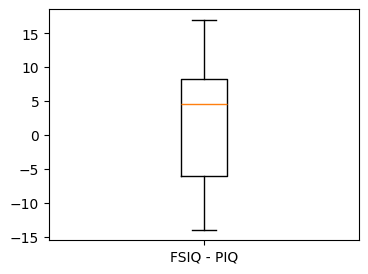
This is equivalent to a one-sample test on the differences between paired observations:

sp.stats.ttest_1samp(data['FSIQ'] - data['PIQ'], 0)

TtestResult(statistic=np.float64(1.7842019405859857), pvalue=np.float64(0.08217263818364236), df=np.int64(39))

Accordingly, we can perform a nonparametric version of the test with wilcoxon.

sp.stats.wilcoxon(data['FSIQ'], data['PIQ'], method="approx")

WilcoxonResult(statistic=np.float64(274.5), pvalue=np.float64(0.10659492713506856))

Exercise 60

• Test the difference between weights in males and females.

• Use non parametric statistics to test the difference between VIQ in males and females.

Solution to Exercise 60

Conclusion: we find that the data does not support the hypothesis that males and females have different VIQ.

Linear models, multiple factors, and analysis of variance

“formulas” to specify statistical models in Python

A simple linear regression

Note

From an original example by Thomas Haslwanter.

Given two set of observations, x and y, we want to test the hypothesis that y is a linear function of x. In other terms:

\[ y = x * \textit{coef} + \textit{intercept} + e \]

where \(e\) is observation noise. We will use the statsmodels module to:

1. Fit a linear model. We will use the simplest strategy, ordinary least squares (OLS).

2. Test that coef is non zero.

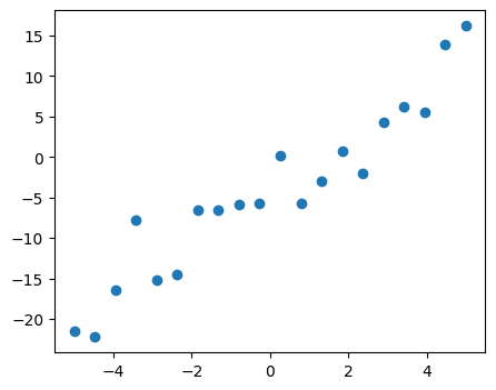
First, we generate simulated data according to the model:

x = np.linspace(-5, 5, 20)

# To get reproducible values, provide a seed value
rng = np.random.default_rng(27446968)

# normal distributed noise
y = -5 + 3 * x + 4 * rng.normal(size=x.shape)

# Create a data frame containing all the relevant variables
data = pd.DataFrame({'x': x, 'y': y})

# Plot the data
plt.figure(figsize=(5, 4))
plt.plot(x, y, "o");

“formulas” for statistics in Python

See the statsmodels documentation

Then we specify an OLS model and fit it:

import statsmodels.formula.api as smf
model = smf.ols("y ~ x", data).fit()

We can inspect the various statistics derived from the fit:

model.summary()

OLS Regression Results

Dep. Variable:	y	R-squared:	0.901
Model:	OLS	Adj. R-squared:	0.896
Method:	Least Squares	F-statistic:	164.5
Date:	Tue, 30 Sep 2025	Prob (F-statistic):	1.72e-10
Time:	18:11:00	Log-Likelihood:	-51.758
No. Observations:	20	AIC:	107.5
Df Residuals:	18	BIC:	109.5
Df Model:	1
Covariance Type:	nonrobust

	coef	std err	t	P>|t|	[0.025	0.975]
Intercept	-4.2948	0.759	-5.661	0.000	-5.889	-2.701
x	3.2060	0.250	12.825	0.000	2.681	3.731

Omnibus:	1.218	Durbin-Watson:	1.796
Prob(Omnibus):	0.544	Jarque-Bera (JB):	0.999
Skew:	0.503	Prob(JB):	0.607
Kurtosis:	2.568	Cond. No.	3.03

Notes:
[1] Standard Errors assume that the covariance matrix of the errors is correctly specified.

Terminology:

Statsmodels uses a statistical terminology: the y variable in statsmodels is called ‘endogenous’ while the x variable is called exogenous. This is discussed in more detail here.

To simplify, y (endogenous) is the value you are trying to predict, while x (exogenous) represents the features you are using to make the prediction.

If the terminology is unfamiliar, you might be able to remember which way round these go by noticing that there is an x in exogenous.

Exercise 61

Retrieve the estimated parameters from the model above.

Hint: use tab-completion to find the relevant attribute.

Categorical variables: comparing groups or multiple categories

Let us go back the data on brain size:

data = pd.read_csv('examples/brain_size.csv', sep=';', na_values=".")

We can write a comparison between IQ of male and female using a linear model:

model = smf.ols("VIQ ~ Gender + 1", data).fit()
model.summary()

OLS Regression Results

Dep. Variable:	VIQ	R-squared:	0.015
Model:	OLS	Adj. R-squared:	-0.010
Method:	Least Squares	F-statistic:	0.5969
Date:	Tue, 30 Sep 2025	Prob (F-statistic):	0.445
Time:	18:11:00	Log-Likelihood:	-182.42
No. Observations:	40	AIC:	368.8
Df Residuals:	38	BIC:	372.2
Df Model:	1
Covariance Type:	nonrobust

	coef	std err	t	P>|t|	[0.025	0.975]
Intercept	109.4500	5.308	20.619	0.000	98.704	120.196
Gender[T.Male]	5.8000	7.507	0.773	0.445	-9.397	20.997

Omnibus:	26.188	Durbin-Watson:	1.709
Prob(Omnibus):	0.000	Jarque-Bera (JB):	3.703
Skew:	0.010	Prob(JB):	0.157
Kurtosis:	1.510	Cond. No.	2.62

Notes:
[1] Standard Errors assume that the covariance matrix of the errors is correctly specified.

Tips on specifying models

Forcing categorical: the ‘Gender’ is automatically detected as a categorical variable, and thus each of its different values are treated as different entities.

An integer column can be forced to be treated as categorical using:

model = ols('VIQ ~ C(Gender)', data).fit()

Intercept: We can remove the intercept using - 1 in the formula, or force the use of an intercept using + 1.

Note

By default, statsmodels treats a categorical variable with K possible values as K-1 ‘dummy’ boolean variables (the last level being absorbed into the intercept term). This is almost always a good default choice - however, it is possible to specify different encodings for categorical variables (https://www.statsmodels.org/devel/contrasts.html).

Link to t-tests between different FSIQ and PIQ

To compare different types of IQ, we need to create a “long-form” table, listing IQs, where the type of IQ is indicated by a categorical variable:

data_fisq = pd.DataFrame({'iq': data['FSIQ'], 'type': 'fsiq'})
data_piq = pd.DataFrame({'iq': data['PIQ'], 'type': 'piq'})
data_long = pd.concat((data_fisq, data_piq))
data_long

	iq	type
0	133	fsiq
1	140	fsiq
2	139	fsiq
3	133	fsiq
4	137	fsiq
...	...	...
35	128	piq
36	124	piq
37	94	piq
38	74	piq
39	89	piq

80 rows × 2 columns

model = smf.ols("iq ~ type", data_long).fit()
model.summary()

OLS Regression Results

Dep. Variable:	iq	R-squared:	0.003
Model:	OLS	Adj. R-squared:	-0.010
Method:	Least Squares	F-statistic:	0.2168
Date:	Tue, 30 Sep 2025	Prob (F-statistic):	0.643
Time:	18:11:00	Log-Likelihood:	-364.35
No. Observations:	80	AIC:	732.7
Df Residuals:	78	BIC:	737.5
Df Model:	1
Covariance Type:	nonrobust

	coef	std err	t	P>|t|	[0.025	0.975]
Intercept	113.4500	3.683	30.807	0.000	106.119	120.781
type[T.piq]	-2.4250	5.208	-0.466	0.643	-12.793	7.943

Omnibus:	164.598	Durbin-Watson:	1.531
Prob(Omnibus):	0.000	Jarque-Bera (JB):	8.062
Skew:	-0.110	Prob(JB):	0.0178
Kurtosis:	1.461	Cond. No.	2.62

Notes:
[1] Standard Errors assume that the covariance matrix of the errors is correctly specified.

We can see that we retrieve the same values for t-test and corresponding p-values for the effect of the type of iq than the previous t-test:

sp.stats.ttest_ind(data['FSIQ'], data['PIQ'])

TtestResult(statistic=np.float64(0.465637596380964), pvalue=np.float64(0.6427725009414841), df=np.float64(78.0))

Multiple Regression: including multiple factors

Note

From an original example by Thomas Haslwanter

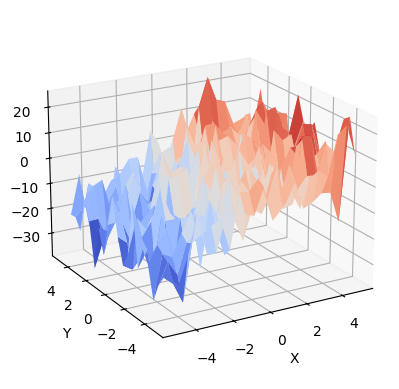
Consider a linear model explaining a variable z (the dependent variable) with 2 variables x and y:

\[ z = x \, c_1 + y \, c_2 + i + e \]

Such a model can be seen in 3D as fitting a plane to a cloud of (x, y, z) points.

# Generate and show the data
x = np.linspace(-5, 5, 21)
# We generate a 2D grid
X, Y = np.meshgrid(x, x)

# To get reproducible values, provide a seed value
rng = np.random.default_rng(27446968)

# Z is the elevation of this 2D grid
Z = -5 + 3 * X - 0.5 * Y + 8 * rng.normal(size=X.shape)

# Plot the data
ax = plt.figure().add_subplot(projection="3d")
surf = ax.plot_surface(X, Y, Z, cmap="coolwarm", rstride=1, cstride=1)
ax.view_init(20, -120)
ax.set_xlabel("X")
ax.set_ylabel("Y")
ax.set_zlabel("Z");

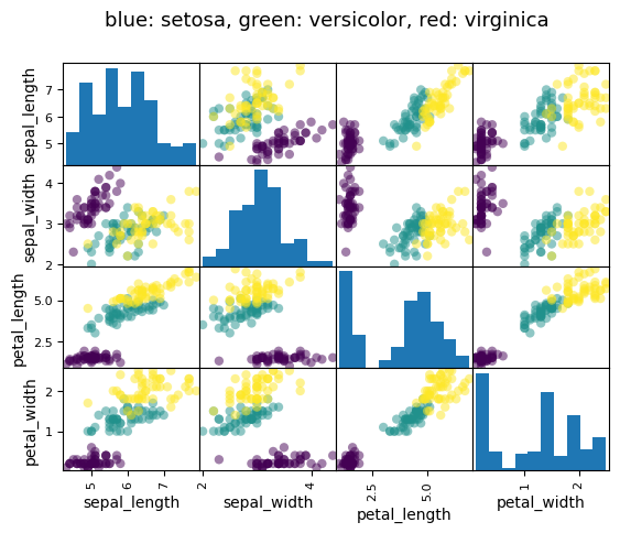
Example: the iris data (examples/iris.csv)

Note

Sepal and petal size tend to be related: bigger flowers are bigger! But is there in addition a systematic effect of species?

data = pd.read_csv('examples/iris.csv')
# Express the names as categories
categories = pd.Categorical(data["name"])
# The parameter 'c' is passed to plt.scatter and will control the color
pd.plotting.scatter_matrix(data, c=categories.codes, marker="o")
fig = plt.gcf()
fig.suptitle("blue: setosa, green: versicolor, red: virginica", size=13);

Let us try to explain the sepal length as a function of the petal width and the category of iris

model = smf.ols("sepal_width ~ name + petal_length", data).fit()
model.summary()

OLS Regression Results

Dep. Variable:	sepal_width	R-squared:	0.478
Model:	OLS	Adj. R-squared:	0.468
Method:	Least Squares	F-statistic:	44.63
Date:	Tue, 30 Sep 2025	Prob (F-statistic):	1.58e-20
Time:	18:11:01	Log-Likelihood:	-38.185
No. Observations:	150	AIC:	84.37
Df Residuals:	146	BIC:	96.41
Df Model:	3
Covariance Type:	nonrobust

	coef	std err	t	P>|t|	[0.025	0.975]
Intercept	2.9813	0.099	29.989	0.000	2.785	3.178
name[T.versicolor]	-1.4821	0.181	-8.190	0.000	-1.840	-1.124
name[T.virginica]	-1.6635	0.256	-6.502	0.000	-2.169	-1.158
petal_length	0.2983	0.061	4.920	0.000	0.178	0.418

Omnibus:	2.868	Durbin-Watson:	1.753
Prob(Omnibus):	0.238	Jarque-Bera (JB):	2.885
Skew:	-0.082	Prob(JB):	0.236
Kurtosis:	3.659	Cond. No.	54.0

Notes:
[1] Standard Errors assume that the covariance matrix of the errors is correctly specified.

Post-hoc hypothesis testing: analysis of variance (ANOVA)

In the above iris example, we wish to test if the petal length is different between versicolor and virginica, after removing the effect of sepal width. This can be formulated as testing the difference between the coefficient associated to versicolor and virginica in the linear model estimated above (it is an Analysis of Variance, ANOVA). For this, we write a vector of ‘contrast’ on the parameters estimated: we want to test "name[T.versicolor] - name[T.virginica]", with an F-test:

print(model.f_test([0, 1, -1, 0]))

<F test: F=3.2453353465742247, p=0.07369058781700905, df_denom=146, df_num=1>

Is this difference significant?

Exercise 62

Going back to the brain size + IQ data, test if the VIQ of male and female are different after removing the effect of brain size, height and weight.

More visualization: Seaborn for statistical exploration

Seaborn combines simple statistical fits with plotting on pandas dataframes.

import seaborn

Let us consider a data giving wages and many other personal information on 500 individuals (Berndt, ER. The Practice of Econometrics. 1991. NY: Addison-Wesley).

We first load and arrange the data — view the code for details:

Show code cell source

Hide code cell source

data = pd.read_csv("examples/wages.txt",
    skiprows=27,
    skipfooter=6,
    sep=None,
    header=None,
    engine="python"  # To allow use of skipfooter.
)
# Give names to the columns
names = [
    "education: Number of years of education",
    "south: 1=person lives in South, 0=Person lives elsewhere",
    "sex: 1=female, 0=Male",
    "experience: Number of years of work experience",
    "union: 1=union member, 0=Not union member",
    "wage: wage (dollars per hour)",
    "age: years",
    "race: 1=other, 2=Hispanic, 3=White",
    "occupation: 1=Management, 2=Sales, 3=Clerical, 4=Service, 5=Professional, 6=Other",
    "sector: 0=Other, 1=Manufacturing, 2=Construction",
    "marr: 0=unmarried,  1=Married",
]
short_names = [n.split(":")[0] for n in names]
data.columns = pd.Index(short_names)
# Log-transform the wages, because they typically are increased with
# multiplicative factors
data["wage"] = np.log10(data["wage"])
# Convert genders to strings (this is particularly useful so that the
# statsmodels formulas detects that `sex` is a categorical variable)
data["sex"] = np.choose(data['sex'], ["male", "female"])

Here are the resulting loaded data.

data

	education	south	sex	experience	union	wage	age	race	occupation	sector	marr
0	8	0	female	21	0	0.707570	35	2	6	1	1
1	9	0	female	42	0	0.694605	57	3	6	1	1
2	12	0	male	1	0	0.824126	19	3	6	1	0
3	12	0	male	4	0	0.602060	22	3	6	0	0
4	12	0	male	17	0	0.875061	35	3	6	0	1
...	...	...	...	...	...	...	...	...	...	...	...
529	18	0	male	5	0	1.055378	29	3	5	0	0
530	12	0	female	33	0	0.785330	51	1	5	0	1
531	17	0	female	25	1	1.366423	48	1	5	0	1
532	12	1	male	13	1	1.298416	31	3	5	0	1
533	16	0	male	33	0	1.186956	55	3	5	1	1

534 rows × 11 columns

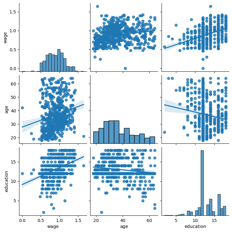
Pairplot: scatter matrices

We can easily have an intuition on the interactions between continuous variables using seaborn.pairplot() to display a scatter matrix:

seaborn.pairplot(data, vars=['wage', 'age', 'education'], kind='reg');

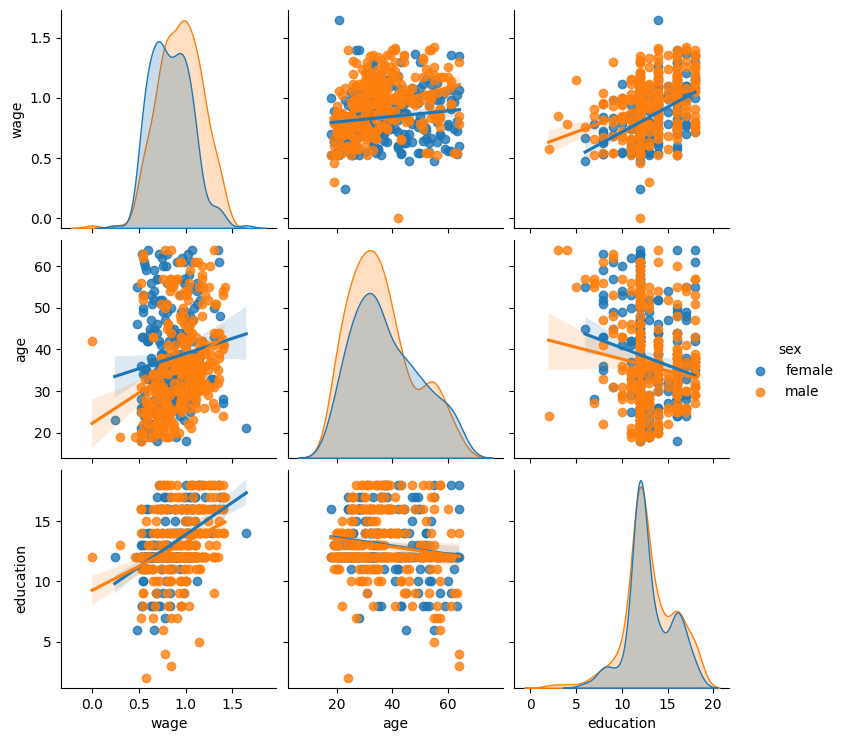
Categorical variables can be plotted as the hue:

seaborn.pairplot(data, vars=['wage', 'age', 'education'],
                 kind='reg', hue='sex');

Look and feel and matplotlib settings

Seaborn changes the default of matplotlib figures to achieve a more “modern”, “excel-like” look. It does that upon import. You can reset the default using:

plt.rcdefaults()

Note

To switch back to seaborn settings, or understand better styling in seaborn, see the relevant section of the seaborn documentation.

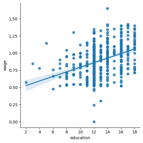
lmplot: plotting a univariate regression

A regression capturing the relation between one variable and another, eg wage, and education, can be plotted using seaborn.lmplot():

seaborn.lmplot(y='wage', x='education', data=data);

Robust regression

Note

Given that, in the above plot, there seems to be a couple of data points that are outside of the main cloud to the right, they might be outliers, not representative of the population, but driving the regression.

To compute a regression that is less sensitive to outliers, one must use a robust model. This is done in seaborn using robust=True in the plotting functions, or in statsmodels by replacing the use of the OLS by a “Robust Linear Model”, statsmodels.formula.api.rlm(). ::::

Testing for interactions

seaborn.lmplot(y="wage", x="education", hue="sex", data=data);

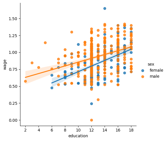
We can first ask do education and sex separately contribute to wage:

result = smf.ols(formula="wage ~ education + sex", data=data).fit()
result.summary()

OLS Regression Results

Dep. Variable:	wage	R-squared:	0.193
Model:	OLS	Adj. R-squared:	0.190
Method:	Least Squares	F-statistic:	63.42
Date:	Tue, 30 Sep 2025	Prob (F-statistic):	2.01e-25
Time:	18:11:07	Log-Likelihood:	86.654
No. Observations:	534	AIC:	-167.3
Df Residuals:	531	BIC:	-154.5
Df Model:	2
Covariance Type:	nonrobust

	coef	std err	t	P>|t|	[0.025	0.975]
Intercept	0.4053	0.046	8.732	0.000	0.314	0.496
sex[T.male]	0.1008	0.018	5.625	0.000	0.066	0.136
education	0.0334	0.003	9.768	0.000	0.027	0.040

Omnibus:	4.675	Durbin-Watson:	1.792
Prob(Omnibus):	0.097	Jarque-Bera (JB):	4.876
Skew:	-0.147	Prob(JB):	0.0873
Kurtosis:	3.365	Cond. No.	69.7

Notes:
[1] Standard Errors assume that the covariance matrix of the errors is correctly specified.

Our next question is — do wages increase more with education for males than females?

Note

The plot above is made of two different fits. We need to formulate a single model that tests for a variance of slope across the two populations. This is done via an “interaction”.

result = smf.ols(formula='wage ~ education + sex + education * sex',
                 data=data).fit()
result.summary()

OLS Regression Results

Dep. Variable:	wage	R-squared:	0.198
Model:	OLS	Adj. R-squared:	0.194
Method:	Least Squares	F-statistic:	43.72
Date:	Tue, 30 Sep 2025	Prob (F-statistic):	2.94e-25
Time:	18:11:07	Log-Likelihood:	88.503
No. Observations:	534	AIC:	-169.0
Df Residuals:	530	BIC:	-151.9
Df Model:	3
Covariance Type:	nonrobust

	coef	std err	t	P>|t|	[0.025	0.975]
Intercept	0.2998	0.072	4.173	0.000	0.159	0.441
sex[T.male]	0.2750	0.093	2.972	0.003	0.093	0.457
education	0.0415	0.005	7.647	0.000	0.031	0.052
education:sex[T.male]	-0.0134	0.007	-1.919	0.056	-0.027	0.000

Omnibus:	4.838	Durbin-Watson:	1.825
Prob(Omnibus):	0.089	Jarque-Bera (JB):	5.000
Skew:	-0.156	Prob(JB):	0.0821
Kurtosis:	3.356	Cond. No.	194.

Notes:
[1] Standard Errors assume that the covariance matrix of the errors is correctly specified.

Can we conclude that education benefits males more than females?

Take home messages

• Hypothesis testing and p-values give you the significance of an effect / difference.

• Formulas (with categorical variables) enable you to express rich links in your data.

• Visualizing your data and fitting simple models give insight into the data.

• Conditionning (adding factors that can explain all or part of the variation) is an important modeling aspect that changes the interpretation.