Population and permutation¶

Here we analyze the Brexit survey.

As you will see in the link above, the data are from a survey of the UK population. Each row in the survey corresponds to one person answering. One of the questions, named cut15 is how the person voted in the Brexit referendum. Another, numage is the age of the person in years.

# Array library.
import numpy as np

# Data frame library.
import pandas as pd

# Plotting
import matplotlib.pyplot as plt
%matplotlib inline

# Fancy plots
plt.style.use('fivethirtyeight')

If you are running on your laptop, first download the data file to the same directory as this notebook.

The cell below loads the data file into memory with Pandas. Notice the .tab extension for this file. This file is just like the .csv (Comma Separated Values) files you have already seen, but the values are separated by a different character. Instead of being separated by commas - , - they are separated by a character called Tab. We tell Pandas about this in the cell below:

# Load the data frame, and put it in the variable "audit_data".
# The values are separated by tab characters, written as "\t" in Python
# strings.
audit_data = pd.read_csv('audit_of_political_engagement_14_2017.tab',
                         sep='\t')
# Show the first 5 rows.
audit_data.head()

	cu044	cu045	cu046	cu047	cu0410	...	intten	cx_971_980	serial	week	wts	numage	weight0	sgrade_grp	age_grp	region2
0	0	1	1	0	0	...	-1	3.41659	1399	648	3.41659	37	3.41659	1	4	3
1	0	0	0	0	1	...	-1	2.68198	1733	648	2.68198	55	2.68198	2	6	3
2	0	1	0	0	0	...	-1	0.79379	1736	648	0.79379	71	0.79379	2	7	4
3	0	1	0	1	0	...	-1	1.40580	1737	648	1.40580	37	1.40580	1	4	4
4	1	1	0	1	0	...	-1	0.89475	1738	648	0.89475	42	0.89475	2	4	4

5 rows × 370 columns

Now get the ages for the Leavers and the Remainers.

A small number of ages are recorded as 0, meaning we do not have the correct age for that person / row. First we drop rows with ages recorded as 0, then select the remaining rows corresponding to people who voted to remain (cut15 value of 1) and leave (cut15 value of 2):

# Drop rows where age is 0
good_data = audit_data[audit_data['numage'] != 0]
# Get data frames for leavers and remainers
remain_ages = good_data[good_data['cut15'] == 1]['numage']
leave_ages = good_data[good_data['cut15'] == 2]['numage']

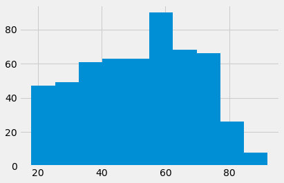
Show the age distributions for the two groups:

remain_ages.hist()
len(remain_ages)

../_images/population_permutation_7_1.png

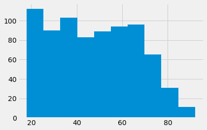
leave_ages.hist()
len(leave_ages)

../_images/population_permutation_8_1.png

These certainly look like different distributions.

We might summarize the difference, by looking at the difference in means:

leave_mean = np.mean(leave_ages)
leave_mean

51.715341959334566

remain_mean = np.mean(remain_ages)
remain_mean

48.01550387596899

difference = leave_mean - remain_mean
difference

3.6998380833655773

The distributions do look different.

They have a mean difference of nearly 4 years.

Could this be due to sampling error?

If we took two random samples of 774 and 541 voters, from the same population, we would expect to see some difference, just by chance.

By chance means, because random samples vary.

What is the population, in this case?

It is not exactly the whole UK population, because the survey only sampled people who were eligible to vote.

It might not even be the whole UK population, who are eligible to vote. Perhaps the survey company got a not-representative range of ages, for some reason. We are not interested in that question, only the question of whether the Leave and Remain voters could come from the same population, where the population is, people selected by the survey company.

How do we find this population, to do our simulation?

Population by permutation¶

Here comes a nice trick. We can use the data that we already have, to simulate the effect of drawing lots of random samples, from the underlying population.

Let us assume that the Leave voters and the Remain voters are in fact samples from the same underlying population.

If that is the case, we can throw the Leave and Remain voters into one big pool of 774 + 541 == 1315 voters.

Then we can take split this new mixed sample into two groups, at random, one with 774 voters, and the other with 541. The new groups have a random mix of the original Leave and Remain voters. Then we calculate the difference in means between these two new, fake groups.

pooled = np.append(remain_ages, leave_ages)
pooled

array([37, 55, 37, ..., 20, 40, 31])

len(pooled)

We mix the two samples together, using np.random.permutation, to make a random permutation of the values. It works like this:

pets = np.array(['cat', 'dog', 'rabbit'])
pets

array(['cat', 'dog', 'rabbit'], dtype='<U6')

np.random.permutation(pets)

array(['rabbit', 'cat', 'dog'], dtype='<U6')

np.random.permutation(pets)

array(['rabbit', 'dog', 'cat'], dtype='<U6')

Now to mix up ages of the Leavers and Remainers:

shuffled = np.random.permutation(pooled)
shuffled

array([71, 27, 68, ..., 61, 20, 29])

We split the newly mixed group into 774 simulated Remain voters and 541 simulated Leave voters, where each group is a random mix of the original Leave and Remain ages.

# The first 774 values
fake_remainers = shuffled[:774]
# The rest
fake_leavers = shuffled[774:]
len(fake_leavers)

Now we can calculate the mean difference. This is our first simulation:

fake_difference = np.mean(fake_leavers) - np.mean(fake_remainers)
fake_difference

0.4966112138016001

That looks a lot smaller than the difference we saw. We want to keep doing this, to collect more simulations. We need to mix up the ages again, to give us new random samples of fake Remainers and fake Leavers.

shuffled = np.random.permutation(pooled)
fake_difference_2 = np.mean(shuffled[:774]) - np.mean(shuffled[774:])
fake_difference_2

-0.9990781737332028

We want to keep doing this - and that calls for a for loop. That’s what we will do in the next page.

Coding for Data - 2020 edition

Population and permutation¶

Population by permutation¶