The law of large numbers¶

# Don't change this cell; just run it.
import numpy as np
import matplotlib.pyplot as plt
# Make the plots look more fancy.
plt.style.use('fivethirtyeight')

You have already seen the law of large numbers in action, in the central limit theorem page.

The law of large numbers says that, as you take more and more samples, the average of the samples will get closer and closer to the expected result.

In this page, we look at probabilities and proportions.

Consider the set up in the first Bayes page. We are playing a game where I offer you a box which has a 30% chance of being a BOX4 type box, and a 70% chance of being a BOX2 type box. BOX4 boxes have four box4 balls and one box2; BOX2 boxes have two box4 and three box2 — but that does not matter for our purpose.

p_box4 = 0.3
p_box2 = 0.7

Here we think about what happens as we take samples with larger and larger number of boxes, and take the proportion (this is also an average) of BOX4s in the sample.

The law of large numbers says that, as we take more samples of the boxes, the proportion of BOX4s in the sample will get closer and closer to the probability of getting BOX4 on any one trial.

Let’s start by taking samples of 100 boxes. One sample will be one trial.

Here’s one trial, taking 100 boxes:

boxes = np.random.choice(['box4', 'box2'],
                          p=[p_box4, p_box2],
                          size=100)
prop = np.count_nonzero(boxes == 'box4') / 100
print('Proportion of BOX4', prop)

Proportion of BOX4 0.35

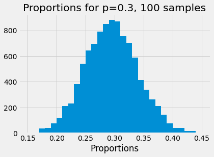
Now we run 1000 trials. On each trial we get 100 boxes, and record the proportion of BOX4. Finally we show the spread of proportions that we get.

n_iters = 10000
n_boxes = 100
props = np.zeros(n_iters)
for i in np.arange(n_iters):
    samples = np.random.choice(['box4', 'box2'],
                               p=[p_box4, p_box2],
                               size=n_boxes)
    props[i] = np.count_nonzero(samples == 'box4') / n_boxes
# Define the bins for the histogram to make them comparable across n_boxes
plt.hist(props, bins=np.arange(0.15, 0.45, 0.01))
plt.xlabel('Proportions')
plt.title('Proportions for p=0.3, ' +  str(n_boxes) + ' samples');

Because we want to repeat this several times with different numbers of boxes, we make the code above into a function:

def show_proportions(n_boxes, n_iters=10000):
    props = np.zeros(n_iters)
    for i in np.arange(n_iters):
        samples = np.random.choice(['box4', 'box2'],
                                   p=[p_box4, p_box2],
                                   size=n_boxes)
        props[i] = np.count_nonzero(samples == 'box4') / n_boxes
    # Define the bins for the histogram to make them comparable across n_boxes
    plt.hist(props, bins=np.arange(0.15, 0.45, 0.01))
    plt.xlabel('Proportions')
    plt.title('Proportions for p=0.3, ' +  str(n_boxes) + ' samples');

Here is the spread (distribution) we saw above, for 100 box samples, but using the function.

show_proportions(100)

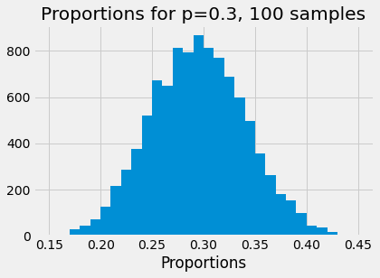
The law of large numbers says that, the larger the number boxes in our sample, the closer the proportions become, to the expected proportion — which is the probability, 0.3.

Here we increase the number of boxes in the sample to 1000.

show_proportions(1000)

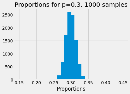
Notice that the distribution has got considerably tighter; the proportions do still vary from trial to trial, but they vary less than for the case with 100 boxes, and they are, on average, a lot close to the expected value of 0.3.

Here is the result of trials taking proportions of 10000 boxes:

show_proportions(10000)

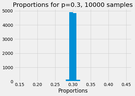
Now the distribution is getting very tight around the expected value.

In fact, the law of large numbers tells us that, as the number of boxes in our sample gets very high, the proportion of BOX4 in the sample gets very close to 0.3.

Another way of saying this, is that in the long run, if we take huge numbers of boxes in our sample, our proportions will get closer and closer to the probability on the single trial — of 0.3.

One useful way to think of this, is of each individual box in the sample flowing along one of two paths. There is a probability of 0.3 that the box will flow along the BOX4 path, and a probability of 0.7 that it will flow along the BOX2 path. In the long run, 30% of the boxes end up at the end of the BOX4 path, and 70% of trials end up at the end of the BOX2 path.

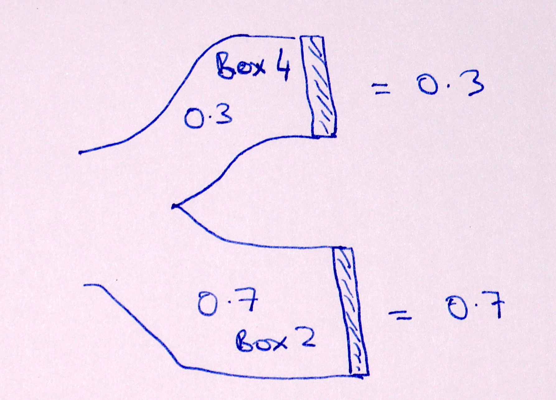
These diagrams of flow can be called Sankey diagrams. They are useful for thinking about probability.

Coding for Data - 2020 edition

The law of large numbers¶