Introduction to data frames
Pandas is a Python package that implements data frames, and functions that operate on data frames.
# Load the Pandas data science library, call it 'pd'
import pandas as pd
# Turn on a setting to use Pandas more safely.
# We will discuss this setting later.
pd.set_option('mode.chained_assignment', 'raise')
We will also use the usual Numpy array library:
# Load the Numpy array library, call it 'np'
import numpy as np
Data frames and series
We start by loading data from a Comma Separated Value file (CSV
file). If you are running on your laptop, you should download
the gender_stats.csv
file to the same directory as this notebook.
See the gender statistics description page for more detail on the dataset.
# Load the data file
gender_data = pd.read_csv('gender_stats.csv')
This is our usual assignment statement. The LHS is gender_data, the variable name. The RHS is an expression, that returns a value.
What type of value does it return?
type(gender_data)
pandas.core.frame.DataFrame
Pandas integrates with the Notebook, so, if you display a data frame in the notebook, it does a nice display of rows and columns.
gender_data
| country_name | country_code | fert_rate | gdp_us_billion | health_exp_per_cap | health_exp_pub | prim_ed_girls | mat_mort_ratio | population | |
|---|---|---|---|---|---|---|---|---|---|
| 0 | Aruba | ABW | 1.66325 | NaN | NaN | NaN | 48.721939 | NaN | 0.103744 |
| 1 | Afghanistan | AFG | 4.95450 | 19.961015 | 161.138034 | 2.834598 | 40.109708 | 444.00 | 32.715838 |
| 2 | Angola | AGO | 6.12300 | 111.936542 | 254.747970 | 2.447546 | NaN | 501.25 | 26.937545 |
| 3 | Albania | ALB | 1.76925 | 12.327586 | 574.202694 | 2.836021 | 47.201082 | 29.25 | 2.888280 |
| 4 | Andorra | AND | NaN | 3.197538 | 4421.224933 | 7.260281 | 47.123345 | NaN | 0.079547 |
| ... | ... | ... | ... | ... | ... | ... | ... | ... | ... |
| 211 | Kosovo | XKX | 2.14250 | 6.804620 | NaN | NaN | NaN | NaN | 1.813820 |
| 212 | Yemen, Rep. | YEM | 4.22575 | 36.819337 | 207.949700 | 1.417836 | 44.470076 | 399.75 | 26.246608 |
| 213 | South Africa | ZAF | 2.37525 | 345.209888 | 1123.142656 | 4.241441 | 48.516298 | 143.75 | 54.177209 |
| 214 | Zambia | ZMB | 5.39425 | 24.280990 | 185.556359 | 2.687290 | 49.934484 | 233.75 | 15.633220 |
| 215 | Zimbabwe | ZWE | 3.94300 | 15.495514 | 115.519881 | 2.695188 | 49.529875 | 398.00 | 15.420964 |
216 rows × 9 columns
Notice the NaN at the top of the GDP column. This is a missing value. We
will come to these in missing values.
For the moment, we will do something quick and dirty, which is to drop all the missing values from the data frame. Be careful - this is rarely the right thing to do, without a lot of investigation as to why the values are missing.
# Drop all missing values.  Be careful, this is rarely the right thing to do.
gender_data_no_na = gender_data.dropna()
gender_data_no_na
| country_name | country_code | fert_rate | gdp_us_billion | health_exp_per_cap | health_exp_pub | prim_ed_girls | mat_mort_ratio | population | |
|---|---|---|---|---|---|---|---|---|---|
| 1 | Afghanistan | AFG | 4.95450 | 19.961015 | 161.138034 | 2.834598 | 40.109708 | 444.00 | 32.715838 |
| 3 | Albania | ALB | 1.76925 | 12.327586 | 574.202694 | 2.836021 | 47.201082 | 29.25 | 2.888280 |
| 5 | United Arab Emirates | ARE | 1.79300 | 375.027082 | 2202.407569 | 2.581168 | 48.789260 | 6.00 | 9.080299 |
| 6 | Argentina | ARG | 2.32800 | 550.980968 | 1148.256142 | 2.782216 | 48.915810 | 53.75 | 42.976675 |
| 7 | Armenia | ARM | 1.54550 | 10.885362 | 348.663884 | 1.916016 | 46.782180 | 27.25 | 2.904683 |
| ... | ... | ... | ... | ... | ... | ... | ... | ... | ... |
| 210 | Samoa | WSM | 4.11825 | 0.799887 | 366.353096 | 5.697059 | 48.350049 | 54.75 | 0.192225 |
| 212 | Yemen, Rep. | YEM | 4.22575 | 36.819337 | 207.949700 | 1.417836 | 44.470076 | 399.75 | 26.246608 |
| 213 | South Africa | ZAF | 2.37525 | 345.209888 | 1123.142656 | 4.241441 | 48.516298 | 143.75 | 54.177209 |
| 214 | Zambia | ZMB | 5.39425 | 24.280990 | 185.556359 | 2.687290 | 49.934484 | 233.75 | 15.633220 |
| 215 | Zimbabwe | ZWE | 3.94300 | 15.495514 | 115.519881 | 2.695188 | 49.529875 | 398.00 | 15.420964 |
167 rows × 9 columns
The data frame has rows and columns. Like other Python objects, it has
attributes. These are pieces of data associated with the data frame. You
have already seen methods, which are functions associated with the data
frame. You can access attributes in the same way as you access methods, by
typing the variable name, followed by a dot ., followed by the attribute
name.
For example, one attribute of the data frame, is the shape:
gender_data_no_na.shape
(167, 9)
Another attribute is columns. This has the column names. For
example, here is a good way of quickly seeing the column names
for a data frame:
gender_data_no_na.columns
Index(['country_name', 'country_code', 'fert_rate', 'gdp_us_billion',
       'health_exp_per_cap', 'health_exp_pub', 'prim_ed_girls',
       'mat_mort_ratio', 'population'],
      dtype='object')
You need more information about what these column names refer to. Here are the longer descriptions from the original data source (link above):
fert_rate: Fertility rate, total (births per woman).gdp_us_billion: GDP (in current US $ billions).health_exp_per_cap: Health expenditure per capita, PPP (constant 2011 international $).health_exp_pub: Health expenditure, public (% of GDP).prim_ed_girls: Primary education, pupils (% female).mat_mort_ratio: Maternal mortality ratio (modeled estimate, per 100,000 live births).population: Population, total.
You have seen array slicing (in Selecting with arrays. You remember that array slicing uses square brackets. Data frames also allow slicing. For example, we often want to get all the data for a single column of the data frame. To do this, we use the same square bracket notation as we use for array slicing, with the name of the column inside the square brackets.
gdp = gender_data_no_na['gdp_us_billion']
What type of thing is this column of data?
type(gdp)
pandas.core.series.Series
Here are the values for gdp. You will notice that these are the same values
you saw in the “gdp_us_billion” column when you displayed the whole data
frame.
gdp
1       19.961015
3       12.327586
5      375.027082
6      550.980968
7       10.885362
          ...
210      0.799887
212     36.819337
213    345.209888
214     24.280990
215     15.495514
Name: gdp_us_billion, Length: 167, dtype: float64
Plotting, the basic way
There are two ways of getting plots from data in data frames. Here we use the most basic method, that you have already seen. Soon, we will get onto a more elegant plotting method.
We start with the magic incantation to load the plotting library.
# Load the library for plotting, name it 'plt'
import matplotlib.pyplot as plt
# Display plots inside the notebook.
%matplotlib inline
# Make plots look a little more fancy
plt.style.use('fivethirtyeight')
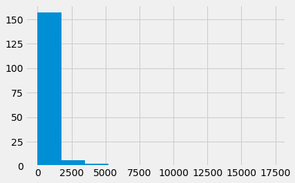
The gdp variable is a sequence of values, so we can do a histogram on these
values, as we have done histograms on arrays.
plt.hist(gdp);
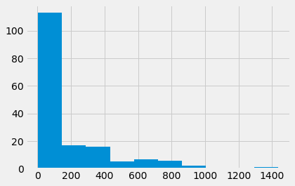
Now we have had a look at the GDP values, we will look at the
values for the mat_mort_ratio column. These are the numbers
of women who die in childbirth for every 100,000 births.
mmr = gender_data_no_na['mat_mort_ratio']
mmr
1      444.00
3       29.25
5        6.00
6       53.75
7       27.25
        ...
210     54.75
212    399.75
213    143.75
214    233.75
215    398.00
Name: mat_mort_ratio, Length: 167, dtype: float64
plt.hist(mmr);
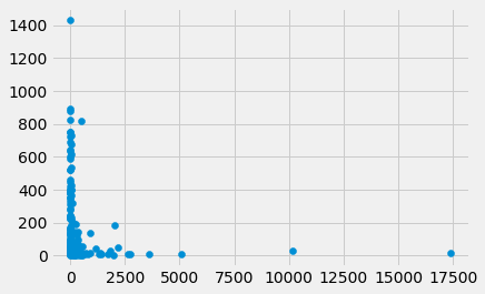
We are interested in the relationship of gpp and mmr. Maybe richer
countries have better health care, and fewer maternal deaths.
Here is a plot, using the standard Matplotlib scatter
function.
plt.scatter(gdp, mmr);
Showing the top 5 values with the head method
We have already seen that Pandas will display the data frame with nice formatting. If the data frame is long, it will display only the first few and the last few rows:
gender_data_no_na
| country_name | country_code | fert_rate | gdp_us_billion | health_exp_per_cap | health_exp_pub | prim_ed_girls | mat_mort_ratio | population | |
|---|---|---|---|---|---|---|---|---|---|
| 1 | Afghanistan | AFG | 4.95450 | 19.961015 | 161.138034 | 2.834598 | 40.109708 | 444.00 | 32.715838 |
| 3 | Albania | ALB | 1.76925 | 12.327586 | 574.202694 | 2.836021 | 47.201082 | 29.25 | 2.888280 |
| 5 | United Arab Emirates | ARE | 1.79300 | 375.027082 | 2202.407569 | 2.581168 | 48.789260 | 6.00 | 9.080299 |
| 6 | Argentina | ARG | 2.32800 | 550.980968 | 1148.256142 | 2.782216 | 48.915810 | 53.75 | 42.976675 |
| 7 | Armenia | ARM | 1.54550 | 10.885362 | 348.663884 | 1.916016 | 46.782180 | 27.25 | 2.904683 |
| ... | ... | ... | ... | ... | ... | ... | ... | ... | ... |
| 210 | Samoa | WSM | 4.11825 | 0.799887 | 366.353096 | 5.697059 | 48.350049 | 54.75 | 0.192225 |
| 212 | Yemen, Rep. | YEM | 4.22575 | 36.819337 | 207.949700 | 1.417836 | 44.470076 | 399.75 | 26.246608 |
| 213 | South Africa | ZAF | 2.37525 | 345.209888 | 1123.142656 | 4.241441 | 48.516298 | 143.75 | 54.177209 |
| 214 | Zambia | ZMB | 5.39425 | 24.280990 | 185.556359 | 2.687290 | 49.934484 | 233.75 | 15.633220 |
| 215 | Zimbabwe | ZWE | 3.94300 | 15.495514 | 115.519881 | 2.695188 | 49.529875 | 398.00 | 15.420964 |
167 rows × 9 columns
Notice the ... in the center of this listing, to show that it has not printed some rows.
Sometimes we do not want to see all these rows, but only - say - the top five rows. The head method of the data frame is a useful way to do this:
gender_data_no_na.head()
| country_name | country_code | fert_rate | gdp_us_billion | health_exp_per_cap | health_exp_pub | prim_ed_girls | mat_mort_ratio | population | |
|---|---|---|---|---|---|---|---|---|---|
| 1 | Afghanistan | AFG | 4.95450 | 19.961015 | 161.138034 | 2.834598 | 40.109708 | 444.00 | 32.715838 |
| 3 | Albania | ALB | 1.76925 | 12.327586 | 574.202694 | 2.836021 | 47.201082 | 29.25 | 2.888280 |
| 5 | United Arab Emirates | ARE | 1.79300 | 375.027082 | 2202.407569 | 2.581168 | 48.789260 | 6.00 | 9.080299 |
| 6 | Argentina | ARG | 2.32800 | 550.980968 | 1148.256142 | 2.782216 | 48.915810 | 53.75 | 42.976675 |
| 7 | Armenia | ARM | 1.54550 | 10.885362 | 348.663884 | 1.916016 | 46.782180 | 27.25 | 2.904683 |
The Series also has a head method, that does the same thing:
gdp.head()
1     19.961015
3     12.327586
5    375.027082
6    550.980968
7     10.885362
Name: gdp_us_billion, dtype: float64
Selecting rows
We often want to select rows from the data frame that match some criterion.
Say we want to select the rows corresponding the countries with a high GDP.
Looking at the histogram of gdp above, we could try this as a threshold to
identify high GDP countries.
high_gdp = gdp > 1000
high_gdp.head()
1    False
3    False
5    False
6    False
7    False
Name: gdp_us_billion, dtype: bool
type(high_gdp)
pandas.core.series.Series
Notice that high_gdp is a Boolean series, like the Boolean arrays you have
already seen. It has True for elements corresponding to countries with
gdp value greater than 1000 and False otherwise.
We can use this Boolean series to select rows from the data frame.
Remember indexing. When we follow a name of something, like an array or series or data frame, with an open square bracket, this means we are trying to get data from the array or Series. The stuff inside the square brackets says what we want.
When we put our Boolean series inside the square brackets, it works like this:
rich_gender_data = gender_data_no_na[high_gdp]
rich_gender_data
| country_name | country_code | fert_rate | gdp_us_billion | health_exp_per_cap | health_exp_pub | prim_ed_girls | mat_mort_ratio | population | |
|---|---|---|---|---|---|---|---|---|---|
| 10 | Australia | AUS | 1.861500 | 1422.994116 | 4256.058988 | 6.292381 | 48.576707 | 6.00 | 23.444560 |
| 26 | Brazil | BRA | 1.795250 | 2198.765606 | 1303.199104 | 3.773473 | 47.784577 | 49.50 | 204.159544 |
| 32 | Canada | CAN | 1.600300 | 1708.473627 | 4616.539134 | 7.546247 | 48.808926 | 7.25 | 35.517119 |
| 35 | China | CHN | 1.558750 | 10182.790479 | 657.748859 | 3.015530 | 46.297964 | 28.75 | 1364.446000 |
| 49 | Germany | DEU | 1.450000 | 3601.226158 | 4909.659884 | 8.542615 | 48.568695 | 6.25 | 81.281645 |
| 58 | Spain | ESP | 1.307500 | 1299.724261 | 2963.832825 | 6.545739 | 48.722231 | 5.00 | 46.553128 |
| 63 | France | FRA | 2.005000 | 2647.649725 | 4387.835406 | 8.920420 | 48.772050 | 8.75 | 66.302099 |
| 67 | United Kingdom | GBR | 1.842500 | 2768.864417 | 3357.983675 | 7.720655 | 48.791809 | 9.25 | 64.641557 |
| 88 | India | IND | 2.449250 | 2019.005411 | 241.572477 | 1.292666 | 49.497234 | 185.25 | 1293.742537 |
| 94 | Italy | ITA | 1.390000 | 2005.983980 | 3266.984094 | 6.984374 | 48.407573 | 4.00 | 60.378795 |
| 97 | Japan | JPN | 1.430000 | 5106.024760 | 3687.126279 | 8.496074 | 48.744199 | 5.75 | 127.297102 |
| 104 | Korea, Rep. | KOR | 1.232000 | 1346.751162 | 2385.447251 | 3.915606 | 48.023388 | 12.00 | 50.727212 |
| 124 | Mexico | MEX | 2.257000 | 1188.802780 | 1081.208948 | 3.225839 | 48.906296 | 40.00 | 124.203450 |
| 164 | Russian Federation | RUS | 1.724500 | 1822.691700 | 1755.506635 | 3.731354 | 48.968070 | 25.25 | 143.793504 |
| 202 | United States | USA | 1.860875 | 17369.124600 | 9060.068657 | 8.121961 | 48.758830 | 14.00 | 318.558175 |
type(rich_gender_data)
pandas.core.frame.DataFrame
rich_gender_data is a new data frame, that is a subset of the original
gender_data_no_na frame. It contains only the rows where the GDP value is
greater than 1000 billion dollars. Check the display of rich_gender_data
above to confirm that the values in the gdp_us_billion column are all
greater than 1000.
We can do a scatter plot of GDP values against maternal mortality rate, and we find, oddly, that for rich countries, there is little relationship between GDP and maternal mortality.
plt.scatter(rich_gender_data['gdp_us_billion'],
            rich_gender_data['mat_mort_ratio'])
<matplotlib.collections.PathCollection at 0x10f7d2bb0>
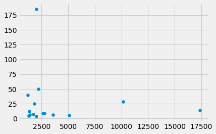
One thing that stands out is the very high value at around 180. Which country does this refer to? We can use sorting to find out.
Sorting data frames
Data frames have a method sort_value. This returns a new data frame with the
rows sorted by the values in the column we specify.
Here are the first five rows of the data frame of the rich countries:
rich_gender_data.head()
| country_name | country_code | fert_rate | gdp_us_billion | health_exp_per_cap | health_exp_pub | prim_ed_girls | mat_mort_ratio | population | |
|---|---|---|---|---|---|---|---|---|---|
| 10 | Australia | AUS | 1.86150 | 1422.994116 | 4256.058988 | 6.292381 | 48.576707 | 6.00 | 23.444560 |
| 26 | Brazil | BRA | 1.79525 | 2198.765606 | 1303.199104 | 3.773473 | 47.784577 | 49.50 | 204.159544 |
| 32 | Canada | CAN | 1.60030 | 1708.473627 | 4616.539134 | 7.546247 | 48.808926 | 7.25 | 35.517119 |
| 35 | China | CHN | 1.55875 | 10182.790479 | 657.748859 | 3.015530 | 46.297964 | 28.75 | 1364.446000 |
| 49 | Germany | DEU | 1.45000 | 3601.226158 | 4909.659884 | 8.542615 | 48.568695 | 6.25 | 81.281645 |
We are interested to find which of these richer countries has a high maternal mortality ratio. To do this, we can make a new data frame where the rows are sorted by the values in the
mat_mort_ratio column:
rich_by_mmr = rich_gender_data.sort_values('mat_mort_ratio')
rich_by_mmr.head()
| country_name | country_code | fert_rate | gdp_us_billion | health_exp_per_cap | health_exp_pub | prim_ed_girls | mat_mort_ratio | population | |
|---|---|---|---|---|---|---|---|---|---|
| 94 | Italy | ITA | 1.3900 | 2005.983980 | 3266.984094 | 6.984374 | 48.407573 | 4.00 | 60.378795 |
| 58 | Spain | ESP | 1.3075 | 1299.724261 | 2963.832825 | 6.545739 | 48.722231 | 5.00 | 46.553128 |
| 97 | Japan | JPN | 1.4300 | 5106.024760 | 3687.126279 | 8.496074 | 48.744199 | 5.75 | 127.297102 |
| 10 | Australia | AUS | 1.8615 | 1422.994116 | 4256.058988 | 6.292381 | 48.576707 | 6.00 | 23.444560 |
| 49 | Germany | DEU | 1.4500 | 3601.226158 | 4909.659884 | 8.542615 | 48.568695 | 6.25 | 81.281645 |
Notice that the rows are in ascending order of mat_mort_ratio. To find the countries with high maternal mortality, we might prefer to sort in descending order. As usual you can explore how
you might do this by looking at the help for the sort_values method with:
rich_by_mmr.sort_values?
in a new cell. If you do that, you discover the ascending argument, that
you can use like this:
rich_by_descending_mmr = rich_gender_data.sort_values('mat_mort_ratio', ascending=False)
rich_by_descending_mmr.head()
| country_name | country_code | fert_rate | gdp_us_billion | health_exp_per_cap | health_exp_pub | prim_ed_girls | mat_mort_ratio | population | |
|---|---|---|---|---|---|---|---|---|---|
| 88 | India | IND | 2.44925 | 2019.005411 | 241.572477 | 1.292666 | 49.497234 | 185.25 | 1293.742537 |
| 26 | Brazil | BRA | 1.79525 | 2198.765606 | 1303.199104 | 3.773473 | 47.784577 | 49.50 | 204.159544 |
| 124 | Mexico | MEX | 2.25700 | 1188.802780 | 1081.208948 | 3.225839 | 48.906296 | 40.00 | 124.203450 |
| 35 | China | CHN | 1.55875 | 10182.790479 | 657.748859 | 3.015530 | 46.297964 | 28.75 | 1364.446000 |
| 164 | Russian Federation | RUS | 1.72450 | 1822.691700 | 1755.506635 | 3.731354 | 48.968070 | 25.25 | 143.793504 |
As you might have guessed by now, Series also have a sort_values method.
For a Series, you don’t have to specify the column to sort from, because you
are using the Series values.
rich_mmr = rich_gender_data['mat_mort_ratio']
type(rich_mmr)
pandas.core.series.Series
rich_mmr.sort_values(ascending=False)
88     185.25
26      49.50
124     40.00
35      28.75
164     25.25
202     14.00
104     12.00
67       9.25
63       8.75
32       7.25
49       6.25
10       6.00
97       5.75
58       5.00
94       4.00
Name: mat_mort_ratio, dtype: float64
Calculation on data frames
We can calculate with Pandas Series, just as we can with arrays.
For example, now we know that India has both a high GDP, and a high maternal mortality ratio, we wonder whether this is because India also has a large population, and therefore, relatively little money per person to spend on health care.
So, we would like know the GDP per capita. Luckily the data frame as a column “population”:
rich_population = rich_by_descending_mmr["population"]
rich_population
88     1293.742537
26      204.159544
124     124.203450
35     1364.446000
164     143.793504
202     318.558175
104      50.727212
67       64.641557
63       66.302099
32       35.517119
49       81.281645
10       23.444560
97      127.297102
58       46.553128
94       60.378795
Name: population, dtype: float64
We can divide the GDP by the population in millions to get US billion dollars per million population.
This works exactly as it does for arrays:
rich_gdp = rich_by_descending_mmr["gdp_us_billion"]
rich_gdp
88      2019.005411
26      2198.765606
124     1188.802780
35     10182.790479
164     1822.691700
202    17369.124600
104     1346.751162
67      2768.864417
63      2647.649725
32      1708.473627
49      3601.226158
10      1422.994116
97      5106.024760
58      1299.724261
94      2005.983980
Name: gdp_us_billion, dtype: float64
gdp_per_million = rich_gdp / rich_population
gdp_per_million
88      1.560593
26     10.769840
124     9.571415
35      7.462949
164    12.675758
202    54.524184
104    26.548890
67     42.834123
63     39.933121
32     48.102821
49     44.305528
10     60.696133
97     40.111084
58     27.919161
94     33.223319
dtype: float64
Notice that the result is elementwise division. Python divides each element
in rich_gdp by the corresponding element in rich_population.
Remember that India is the first country in the rich_by_descending_mmr
data frame. It also has by far the lowest GDP per million population of
any of this selection of rich countries. Here’s a plot of
gdp_per_million against the corresponding values in mat_mort_ratio:
plt.scatter(gdp_per_million, rich_by_descending_mmr['mat_mort_ratio'])
<matplotlib.collections.PathCollection at 0x10f76cdf0>
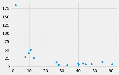
It does look as if low income per person predisposes to high maternal mortality.