Finding lines¶

In The Mean and Slopes, we were looking for the best slope to predict one vector of values from another vector of values.

Specifically, we wanted our slope to predict the Packed Cell Volume (PCV) values from the Hemoglobin (HGB) values.

By analogy with The Mean as Predictor, we decided to choose our line to minimize the average prediction errors, and the sum of squared prediction errors.

We found a solution, by trying many slopes, and choosing the slope giving use the smallest error.

For our question, we were happy to assume that the line passed through 0, 0 — meaning, that when the Hemoglobin is 0, the Packed Cell Volume value is 0. Put another way, we assumed that our line had an intercept value of 0. The intercept is the y value at which the line crosses the y axis, or, put another way, the y value when the x value is 0.

What if we are in a situation where we want to find a line that had a (not zero) intercept, as well as a slope?

import numpy as np
import pandas as pd
import matplotlib.pyplot as plt
%matplotlib inline
# Make plots look a little bit more fancy
plt.style.use('fivethirtyeight')
# Print to 4 decimal places, show tiny values as 0
np.set_printoptions(precision=4, suppress=True)

We return to the students ratings dataset dataset.

This is a dataset, in Excel form, where each row is the average of students’ ratings from <RateMyProfessors.com> across a single subject. Thus, the first row refers to the average of all professors teaching English, the second row refers to all professors teaching Mathematics, and so on.

Download the data file via this link rate_my_course.csv.

Next we load the data.

# Read the data file
ratings = pd.read_csv('rate_my_course.csv')
ratings.head()

	Discipline	Number of Professors	Clarity	Helpfulness	Overall Quality	Easiness
0	English	23343	3.756147	3.821866	3.791364	3.162754
1	Mathematics	22394	3.487379	3.641526	3.566867	3.063322
2	Biology	11774	3.608331	3.701530	3.657641	2.710459
3	Psychology	11179	3.909520	3.887536	3.900949	3.316210
4	History	11145	3.788818	3.753642	3.773746	3.053803

We are interested in the relationship of the “Overall Quality” measure to the “Easiness” measure.

# Convert Easiness and Overall Quality measures to arrays.
easiness = np.array(ratings['Easiness'])
quality = np.array(ratings['Overall Quality'])

Do students rate easier courses as being of better quality?

plt.plot(easiness, quality, 'o')
plt.xlabel('Easiness')
plt.ylabel('Overall Quality')

Text(0, 0.5, 'Overall Quality')

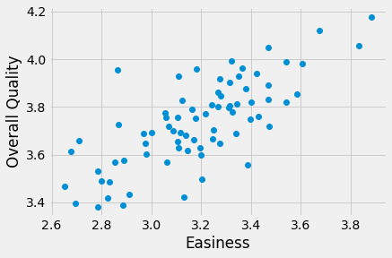
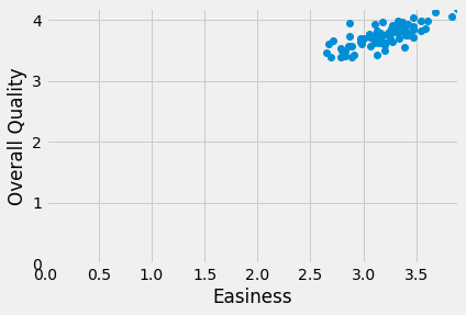
There might be a straight-line relationship here, but it doesn’t look as if it would go through 0, 0:

# The same plot as above, but showing the x, y origin at 0, 0
plt.plot(easiness, quality, 'o')
plt.xlabel('Easiness')
plt.ylabel('Overall Quality')
# Make sure 0, 0 is on the plot.
plt.axis([0, 3.9, 0, 4.2])

(0.0, 3.9, 0.0, 4.2)

In The Mean and Slopes, we assumed that the intercept was zero, so we only had to try different slopes to get our best line.

Here we have a different problem, because we want to find a line that has an intercept that is not zero, so we need to find the best slope and the best intercept at the same time. How do we search for a slope as well as an intercept?

But wait - why do we have to search for the slope and the intercept at the same time? Can’t we just find the best slope, and then the best intercept?

In fact we can’t do that, because the best slope will change for every intercept.

To see why that is, we need to try a few different lines. To do that, we need to remind ourselves about defining lines, and then testing them.

Remember, we can describe a line with an intercept and a slope. Call the intercept \(c\) and a slope \(s\). A line predicts the \(y\) values from the \(x\) values, using the slope \(s\) and the intercept \(c\):

\[ y = c + x * s \]

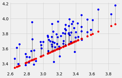
Let’s start with a guess for the line, just from eyeballing the plot. We guess that:

The intercept is around 2.25
The slope is around 0.47

The predicted \(y\) values from this line are (from the formula above):

predicted = 2.25 + easiness * 0.47

where easiness contains our actual \(x\) values.

The prediction error at each point come from the actual \(y\) values minus the predicted \(y\) values.

error = quality - predicted

where quality contains our actual \(y\) values.

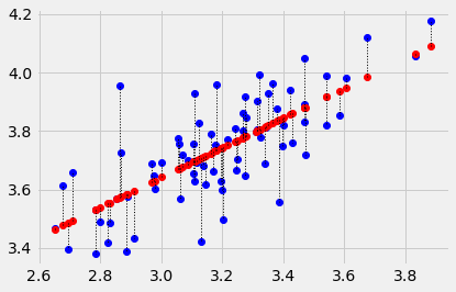
We can look at the predictions for this line (in red), and the actual values (in blue) and then the errors (the lengths of the dotted lines joining the red predictions and the corresponding blue actual values).

# Don't worry about this code, it's just to plot the line, and the errors.
x_values = easiness  # The thing we're predicting from, on the x axis
y_values = quality  # The thing we're predicting, on the y axis.
plt.plot(x_values, y_values, 'o')
plt.plot(x_values, predicted, 'o', color='red')
# Draw a line between predicted and actual
for i in np.arange(len(x_values)):
    x = x_values[i]
    y_0 = predicted[i]
    y_1 = y_values[i]
    plt.plot([x, x], [y_0, y_1], ':', color='black', linewidth=1)

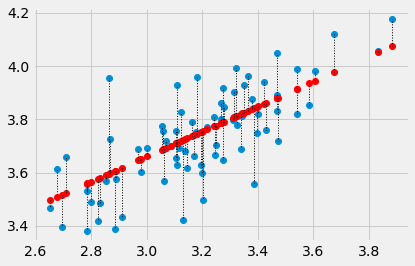
The sum of squared errors is:

# Sum of squared error given c and s
sse_c_s = np.sum(error ** 2)
sse_c_s

1.0849912187001691

Actually, those bits of code are so useful, let’s make them into a function:

def plot_with_errors(x_values, y_values, c, s):
    """ Plot a line through data with errors

    Parameters
    ----------
    x_values : array
        Values we are predicting from, for the x-axis of the plot.
    y_values : array
        Values we are predicting, for the y-axis of the plot.
    c : number
        Intercept for predicting line.
    s : number
        Slope for predicting line.

    Returns
    -------
    s_o_s : number
        The sum of squares of the errors, for the given `x_values`, `y_values` and line.
    """
    # Predict the y values from the line.
    predicted = c + s * x_values
    # Errors are the real values minus the predicted values.
    errors = y_values - predicted
    # Plot real values in blue, predicted values in red.
    plt.plot(x_values, y_values, 'o', color='blue')
    plt.plot(x_values, predicted, 'o', color='red')
    # Draw a line between predicted and actual
    for i in np.arange(len(x_values)):
        x = x_values[i]
        y_0 = predicted[i]
        y_1 = y_values[i]
        plt.plot([x, x], [y_0, y_1], ':', color='black', linewidth=1)
    return np.sum(errors ** 2)

Notice the string at the top of the function, giving details about what the function does, its arguments, and the values it returns. This is called the docstring. It can remind you and other people what the function does, and how to use it. Try making a new cell and type plot_with_errors?. You’ll see this string is the help that Python will fetch for this function.

Now the same thing with the function:

plot_with_errors(easiness, quality, 2.25, 0.47)

1.0849912187001691

If we try a different intercept, we’ll get a different line, and a different error. Let’s try an intercept of 2.1:

plot_with_errors(easiness, quality, 2.1, 0.47)

2.51618856838646

Or, we could go back to the same intercept, but try a different slope, and we’d get a different error. Let’s try a slope of 0.5:

plot_with_errors(easiness, quality, 2.25, 0.5)

1.925931925719183

Now we use the long slow method to find the best slope for our initial intercept of 2.25. You may recognize the following from the mean and slopes notebook.

First we make a function, a bit like the function above, that gives us the error for any given intercept (c) and slope (s) like this:

def sos_error_c_s(c, s):
    predicted = c + easiness * s
    error = quality - predicted
    return np.sum(error ** 2)

We have already calculated the error for the original guess at slope and intercept, but let’s do it again for practice:

# Sum of squared error for our initial guessed line.
predicted = 2.25 + easiness * 0.47
error = quality - predicted
np.sum(error ** 2)

1.0849912187001691

Check that our function gives the same value for the same intercept and slope:

sos_error_c_s(2.25, 0.47)

1.0849912187001691

OK, now we use this function to try lots of different slopes, for this intercept, and see which slope gives us the lowest error. See the means, slopes notebook for the first time we did this.

# Some slopes to try.
some_slopes = np.arange(-2, 2, 0.001)
n_slopes = len(some_slopes)
print('Number of slopes to try:', n_slopes)
# The first 10 slopes to try:
some_slopes[:10]

Number of slopes to try: 4000

array([-2.   , -1.999, -1.998, -1.997, -1.996, -1.995, -1.994, -1.993,
       -1.992, -1.991])

# Try all these slopes for an intercept of 2.25
# For each slope, calculate and record sum of squared error
sos_errors = np.zeros(n_slopes)
for i in np.arange(n_slopes):
    slope = some_slopes[i]
    sos_errors[i] = sos_error_c_s(2.25, slope)

Now plot the errors we got for each slope, and find the slope giving the smallest error:

plt.plot(some_slopes, sos_errors)
plt.xlabel('Candidate slopes')
plt.ylabel('Sum of squared error')

Text(0, 0.5, 'Sum of squared error')

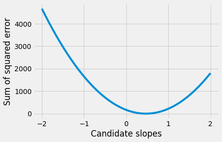
Using the tricks from where and argmin, we find the index (position) of the minimum value, and then find the corresponding slope.

i_of_best_slope = np.argmin(sos_errors)
best_slope_for_2p25 = some_slopes[i_of_best_slope]
print('Best slope for intercept of', 2.25, 'is', best_slope_for_2p25)

Best slope for intercept of 2.25 is 0.4669999999997283

That code also looks useful, so let’s make some of that code into a function we can re-use:

def best_slope_for_intercept(intercept, some_slopes):
    """ Calculate best slope, lowest error for a given intercept

    Parameters
    ----------
    intercept : number
        Intercept.
    some_slopes : array
        Array of candidate slope values to try.

    Returns
    -------
    best_slope : float
        Slope from `some_slopes` that results in lowest error.
    lowest_error : float
        Lowest error score across all slopes in `some_slopes`;
        therefore, error score for `best_slope`.
    """
    n_slopes = len(some_slopes)
    # Try all these slopes, calculate and record sum of squared error
    sos_errors = np.zeros(n_slopes)
    for i in np.arange(n_slopes):
        slope = some_slopes[i]
        sos_errors[i] = sos_error_c_s(intercept, slope)
    i_of_best_slope = np.argmin(sos_errors)
    # Return the slope and associated error as a length 2 array.
    return np.array(
        [some_slopes[i_of_best_slope], sos_errors[i_of_best_slope]]
    )

Now use the function to find the best slope:

best_slope_for_intercept(2.25, some_slopes)

array([0.467 , 1.0768])

OK — that’s the best slope and error for an intercept of 2.25. How about our other suggestion, of an intercept of 2.1? Let’s try that:

best_slope_for_intercept(2.1, some_slopes)

array([0.513 , 1.0677])

Oh dear - the best slope has changed. And, in general, for any intercept, you may able to see that the best slope will be different, as the slope tries to adjust for the stuff that the intercept does not explain.

This means we can’t just find the intercept, and find the best slope for that intercept, at least not in our case - we have to find the best pair of intercept and slope. This is the pair, of all possible pairs, that gives the lowest error.

Our task then, is to find the pair of values — c and s — such that we get the smallest possible value for the sum of squared errors above.

One way of doing this, is to try every possible plausible pair of intercept and slope, calculate the error for this pair, and then find the pair that gave the lowest error.

We are now searching over many combinations of slopes and intercepts.

For example, say we were interested in trying the intercepts 2, 2.1, 2.2. Then we’d run the routine above for each intercept, to find the best slope for each:

print('Best slope, error for 2.0 is ',
      best_slope_for_intercept(2.0, some_slopes))
print('Best slope, error for 2.1 is ',
      best_slope_for_intercept(2.1, some_slopes))
print('Best slope, error for 2.2 is ',
      best_slope_for_intercept(2.2, some_slopes))

Best slope, error for 2.0 is  [0.545  1.0742]
Best slope, error for 2.1 is  [0.513  1.0677]

Best slope, error for 2.2 is  [0.482  1.0712]

From this we conclude that, of the intercepts we have tried, 2.1 is the best, because we could get the lowest error score with that intercept. If this was all we had, we would chose an intercept of 2.1, and its matching best slope of 0.513.

To find out if this is really the best we can do, we can try many intercepts. For each intercept, we find the best slope, with the lowest error. Then we choose the intercept for which we can get the lowest error, and find the best slope for that intercept.

# Some intercepts to try
some_intercepts = np.arange(1, 3.2, 0.01)
n_intercepts = len(some_intercepts)
print('Number of intercepts to try:', n_intercepts)
# First 10 intercepts to try
print('First 10 intercepts', some_intercepts[:10])

Number of intercepts to try: 220
First 10 intercepts [1.   1.01 1.02 1.03 1.04 1.05 1.06 1.07 1.08 1.09]

For each of the 220 possible intercepts, we try all 4000 possible slopes, to find the slope giving the lowest error for that intercept. We store the best slope, and the best error, for each intercept, so we can chose the best intercept, after we have finished.

# An array to collect the best slope found for each intercept.
best_slopes = np.zeros(n_intercepts)
# An array to collect the lowest error found for each intercept.
# This is the error associated with the matching slope above.
lowest_errors = np.zeros(n_intercepts)
# Cycle through each intercept, finding the best slope, and lowest error.
for i in np.arange(n_intercepts):
    # Intercept to try
    intercept = some_intercepts[i]
    # Find best slope, and matching error.
    slope_error = best_slope_for_intercept(intercept, some_slopes)
    # Store the slope and error in their arrays.
    best_slopes[i] = slope_error[0]  # The best slope
    lowest_errors[i] = slope_error[1]  # The matching error
print('First 10 intercepts:\n', some_intercepts[:10])
print('Best slopes for first 10 intercepts:\n', best_slopes[:10])
print('Lowest errors for first 10 intercepts:\n', lowest_errors[:10])

First 10 intercepts:
 [1.   1.01 1.02 1.03 1.04 1.05 1.06 1.07 1.08 1.09]
Best slopes for first 10 intercepts:
 [0.856 0.853 0.85  0.847 0.844 0.841 0.838 0.835 0.831 0.828]
Lowest errors for first 10 intercepts:
 [1.6967 1.6854 1.6742 1.6631 1.6522 1.6414 1.6307 1.6201 1.6097 1.5992]

# Plot the lowest error for each intercept
plt.plot(some_intercepts, lowest_errors)
plt.xlabel('Intercepts')
plt.ylabel('Lowest error for intercept')
plt.title('Lowest error for each intercept')

Text(0.5, 1.0, 'Lowest error for each intercept')

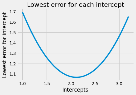
# The lowest error we found for any intercept:
min(lowest_errors)

1.067505831527242

Notice that this error is lower than the error we found for our guessed c and s:

sos_error_c_s(2.25, 0.47)

1.0849912187001691

Again, we use argmin to find the index (position) of the minimum value:

# The index (position) of this lowest error
i_for_lowest = np.argmin(lowest_errors)
i_for_lowest

# The intercept corresponding to the lowest error
best_intercept = some_intercepts[i_for_lowest]
best_intercept

2.120000000000001

# The slope giving the lowest error, for this intercept
best_slope = best_slopes[i_for_lowest]
best_slope

0.5069999999997239

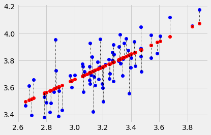
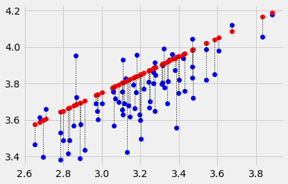
Plot the data, predictions and errors for the line that minimizes the sum of squared error:

plot_with_errors(easiness, quality, best_intercept, best_slope)

1.067505831527242

Now you know about optimization, you will not be surprised to discover that Scipy minimize can also do the search for the intercept and slope pair for us. We send minimize the function we are trying to minimize, and a starting guess for the intercept and slope.

minimize is a little fussy about the functions it will use. It insists that all the parameters need to be passed in as a single argument. In our case, we need to pass both parameters (the intercept and slope) as one value, containing two elements, like this:

def sos_error_for_minimize(c_s):
    # c_s has two elements, the intercept c and the slope s.
    c = c_s[0]
    s = c_s[1]
    predicted = c + easiness * s
    error = quality - predicted
    return np.sum(error ** 2)

This is the form of the function that minimize can use. See using minimize for more detail.

We first confirm this gives us the same answer we got before from our function with two arguments:

# The original function
sos_error_c_s(2.25, 0.47)

1.0849912187001691

# The function in the form that minimize wants
# The two parameters go into a list, that we can pass as a single argument.
sos_error_for_minimize([2.25, 0.47])

1.0849912187001691

As usual with minimize we need to give a starting guess for the intercept and slope. We will start with our initial guess of [2.25, 0.47], but any reasonable guess will do.

from scipy.optimize import minimize
minimize(sos_error_for_minimize, [2.25, 0.47])

      fun: 1.0674471058042072
 hess_inv: array([[ 0.9878, -0.308 ],
       [-0.308 ,  0.0967]])
      jac: array([-0.,  0.])
  message: 'Optimization terminated successfully.'
     nfev: 15
      nit: 3
     njev: 5
   status: 0
  success: True
        x: array([2.1148, 0.5089])

Notice that minimize doesn’t get exactly the same result as we found with the long slow way above. This is because the long slow way only tested intercepts that were step-sizes of 0.01 apart (and slopes that were 0.001 apart). minimize can use much smaller step-sizes, and so finds a more accurate answer.

We won’t spend any time justifying this, but this is also the answer we get from traditional fitting of the least-squares line, as implemented, for example, in the Scipy linregress function:

from scipy.stats import linregress
linregress(easiness, quality)

LinregressResult(slope=0.5088641203940006, intercept=2.114798571643314, rvalue=0.7459725836595872, pvalue=1.5998303978986516e-14, stderr=0.053171209477256925, intercept_stderr=0.1699631063847937)

Notice the values for slope and intercept in the output above.

Coding for Data - 2020 edition

Finding lines¶