\(\newcommand{L}[1]{\| #1 \|}\newcommand{VL}[1]{\L{ \vec{#1} }}\newcommand{R}[1]{\operatorname{Re}\,(#1)}\newcommand{I}[1]{\operatorname{Im}\, (#1)}\)

Fourier without the ei

Introduction

The standard equations for discrete Fourier transforms (DFTs) involve exponentials to the power of \(i\) - the imaginary unit. I personally find these difficult to think about, and it turns out, the DFT is fairly easy to recast in terms of \(\sin\) and \(\cos\). This page goes through this process, and tries to show how thinking in this way can explain some features of the DFT.

How hard is the mathematics?

You will not need heavy math to follow this page. If you don’t remember the following concepts you might want to brush up on them. There are also links to proofs and explanations for these ideas in the page as we go along:

• basic trigonometry (SOH CAH TOA, Pythagoras’ theorem);
• the angle sum rule;
• basic algebra with sums;
• Vectors and dot products;
• vector projection using the dot product.

You will not need to understand complex numbers in any depth, but see Refresher on complex numbers.

Loading and configuring code libraries

Load and configure the Python libraries we will use:

>>> # - compatibility with Python 3
>>> from __future__ import print_function  # print('me') instead of print 'me'
>>> from __future__ import division  # 1/2 == 0.5, not 0

>>> # - import common modules
>>> import numpy as np  # the Python array package
>>> import matplotlib.pyplot as plt  # the Python plotting package

>>> # - tell numpy to print numbers to 4 decimal places only
>>> np.set_printoptions(precision=4, suppress=True)
>>> # - function to print non-numpy scalars to 4 decimal places
>>> def to_4dp(f):
...     return '{0:.4f}'.format(f)

Hint

If running in the IPython console, consider running %matplotlib to enable interactive plots. If running in the Jupyter Notebook, use %matplotlib inline.

Some actual numbers to start

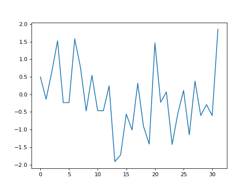
Let us start with a DFT of some data:

>>> # An example input vector
>>> x = np.array(
...     [ 0.4967, -0.1383,  0.6477,  1.523 , -0.2342, -0.2341,  1.5792,
...       0.7674, -0.4695,  0.5426, -0.4634, -0.4657,  0.242 , -1.9133,
...      -1.7249, -0.5623, -1.0128,  0.3142, -0.908 , -1.4123,  1.4656,
...      -0.2258,  0.0675, -1.4247, -0.5444,  0.1109, -1.151 ,  0.3757,
...      -0.6006, -0.2917, -0.6017,  1.8523])
>>> N = 32  # the length of the time-series
>>> plt.plot(x)
[...]

(png, hires.png, pdf)

>>> # Now the DFT
>>> X = np.fft.fft(x)
>>> X
array([-4.3939+0.j    ,  9.0217-3.7036j, -0.5874-6.2268j,  2.5184+3.7749j,
        0.5008-0.8433j,  1.2904-0.4024j,  4.3391+0.8079j, -6.2614+2.1596j,
        1.8974+2.4889j,  0.1042+7.6169j,  0.3606+5.162j ,  4.7965+0.0755j,
       -5.3064-3.2329j,  4.6237+1.5287j, -2.1211+4.4873j, -4.0175-0.3712j,
       -2.0297+0.j    , -4.0175+0.3712j, -2.1211-4.4873j,  4.6237-1.5287j,
       -5.3064+3.2329j,  4.7965-0.0755j,  0.3606-5.162j ,  0.1042-7.6169j,
        1.8974-2.4889j, -6.2614-2.1596j,  4.3391-0.8079j,  1.2904+0.4024j,
        0.5008+0.8433j,  2.5184-3.7749j, -0.5874+6.2268j,  9.0217+3.7036j])

Notice that X - the output of the forward DFT - is a vector of complex numbers. We will go into this in detail later.

When we do the inverse DFT on X we return the original values of our input x, but as complex numbers with imaginary part 0:

>>> # Apply the inverse DFT to the output of the forward DFT
>>> x_back = np.fft.ifft(X)
>>> x_back
array([ 0.4967-0.j, -0.1383-0.j,  0.6477-0.j,  1.5230-0.j, -0.2342-0.j,
       -0.2341+0.j,  1.5792+0.j,  0.7674+0.j, -0.4695-0.j,  0.5426-0.j,
       -0.4634-0.j, -0.4657+0.j,  0.2420-0.j, -1.9133-0.j, -1.7249-0.j,
       -0.5623+0.j, -1.0128-0.j,  0.3142+0.j, -0.9080+0.j, -1.4123+0.j,
        1.4656+0.j, -0.2258+0.j,  0.0675+0.j, -1.4247-0.j, -0.5444+0.j,
        0.1109+0.j, -1.1510+0.j,  0.3757-0.j, -0.6006-0.j, -0.2917-0.j,
       -0.6017-0.j,  1.8523-0.j])

Rewriting the DFT without the \(e^i\)

DFT and FFT

The fast fourier transform (FFT) refers to a particular set of - er - fast algorithms for calculating the DFT. It is common, but confusing, to use “FFT” to mean DFT.

Introducing the discrete Fourier transform

Let us say we have a vector of \(N\) values in time, or space \(\vec{x} = [x_0, x_1 ... x_{N-1}]\). We generally index \(\vec{x}\) with subscript \(n\), so the sample at index \(n\) is \(x_n\).

The DFT converts \(\vec{x}\) from a vector in time, or space, to a vector \(\vec{X}\) representing temporal or spatial frequency components.

We will call our original \(\vec{x}\) the signal, meaning, the signal not transformed to frequency.

The DFT converts \(\vec{x}\) to \(\vec{X}\) where \(\vec{X} = [X_0, X_1, ... X_{N-1}]\). We generally index \(\vec{X}\) with subscript \(k\), so the sample at index \(k\) is \(X_k\).

Here is the equation for the discrete Fourier transform:

\[X_k = \sum_{n=0}^{N-1} x_n \; e^{-i 2 \pi \frac{k}{N} n}\]

This is the transform from signal to frequency. We will call this the forward Fourier transform.

Here is the equation for the inverse Fourier transform:

\[x_n = \frac{1}{N} \sum_{k=0}^{N-1} X_k \; e^{i 2 \pi \frac{k}{N} n}\]

The inverse Fourier transform converts from frequency back to signal.

Scrubbing the \(e^i\)

The forward and inverse equations are very similar; both share a term \(e^{iz}\), where \(z = -2 \pi \frac{k}{N} n\) for the forward transform; \(z = 2 \pi \frac{k}{N} n\) for the inverse transform.

Some people are used to looking at the form \(e^{iz}\) and thinking “aha, that’s a rotation around a circle”. Apparently this is an intuition that builds up over time working with these sorts of equations.

Unfortunately, some of us find it hard to think in complex exponentials, or in terms of complex numbers.

So, in this tutorial, we will express the Fourier transform in terms of \(\sin\) and \(\cos\). We will be using complex numbers, but almost entirely as a pair of numbers to represent two components of the same thing, rather than a single number with a real and imaginary part.

Having said that, we will need some very basic properties of complex and imaginary numbers - see Refresher on complex numbers.

Back to scrubbing the \(e^i\)

Our first tool in this enterprise is Euler’s formula:

\[e^{ix} = \cos x + i\sin x\]

This is the basis for thinking of \(e^{ix}\) as being rotation around a circle, of which you will hear no more in this page. In our case, it allows us to rewrite the forward and inverse Fourier transforms:

First let’s define a new value \(D\), that depends on \(N\) - the number of observations in our vector \(\vec{x}\).

\[D \triangleq \frac{2 \pi}{N}\]

With that value:

\[\begin{split}X_k = \sum_{n=0}^{N-1} x_n \cdot \cos(-k n D) + i \sum_{n=0}^{N-1} x_n \cdot \sin(-k n D) \\ x_n = \frac{1}{N} \sum_{k=0}^{N-1} X_k \cdot \cos(k n D) + i \frac{1}{N} \sum_{k=0}^{N-1} X_k \cdot \sin(k n D)\end{split}\]

We can simplify this a bit further, because, for any angle \(\alpha\):

\[\begin{split}\cos(-\alpha) = cos(\alpha) \\ \sin(-\alpha) = -sin(\alpha)\end{split}\]

\[\begin{split}X_k = \sum_{n=0}^{N-1} x_n \cdot \cos(k n D) - i \sum_{n=0}^{N-1} x_n \cdot \sin(k n D) \\ x_n = \frac{1}{N} \sum_{k=0}^{N-1} X_k \cdot \cos(k n D) + i \frac{1}{N} \sum_{k=0}^{N-1} X_k \cdot \sin(k n D)\end{split}\]

Rewriting as dot products

We can simplify the notation, and maybe make the process clearer, by rewriting these sums in terms of dot products.

As y’all remember, the dot product of two length \(N\) vectors \(\vec{v}, \vec{w}\) is given by:

\[\vec{v} \cdot \vec{w} \triangleq \sum_{i=0}^{N-1} v_i w_i\]

Clearly, because \(v_i w_i = w_i v_i\):

\[\vec{v} \cdot \vec{w} = \vec{w} \cdot \vec{v}\]

For the moment, let us concentrate on the forward transform.

\[\begin{split}\vec{t_k} \triangleq \left[ k 2 \pi \frac{n}{N} \;\mathrm{for}\; n \in 0,1,\ldots,N-1 \right] \\ \vec{c_k} \triangleq \left[ \cos(t_{k,n}) \;\mathrm{for}\; n \in 0,1,\ldots,N-1 \right] \\ \vec{s_k} \triangleq \left[ \sin(t_{k,n}) \;\mathrm{for}\; n \in 0,1,\ldots,N-1 \right]\end{split}\]

Now we can rewrite the sums in the forward transform as the sum of two dot products:

\[X_k = \vec{x} \cdot \vec{c_k} - i \vec{x} \cdot \vec{s_k}\]

The vector \(\vec{t_k}\) is key to understanding what is going on. \(t_k\) sets up the horizontal axis values to sample a \(\sin\) or \(\cos\) function so the function gives us \(k\) cycles over the indices \(0 .. N-1\).

In the formulae above, \(n / N\) is the proportion of the whole signal width \(N\), so it varies between 0 and \((N-1) / N\). The \(2 \pi\) corresponds to one cycle of the cosine or sine function.

So, \(\vec{t_0}\) gives a vector of zeros corresponding to \(k=0\) cycles across \(0 ... N-1\). \(\vec{t_1}\) gives us \(0\) up to (not including) \(2 \pi\) - one cycle across the indices \(0 .. N-1\). \(\vec{t_2}\) gives us \(0\) up to (not including) \(4 \pi\) - two cycles.

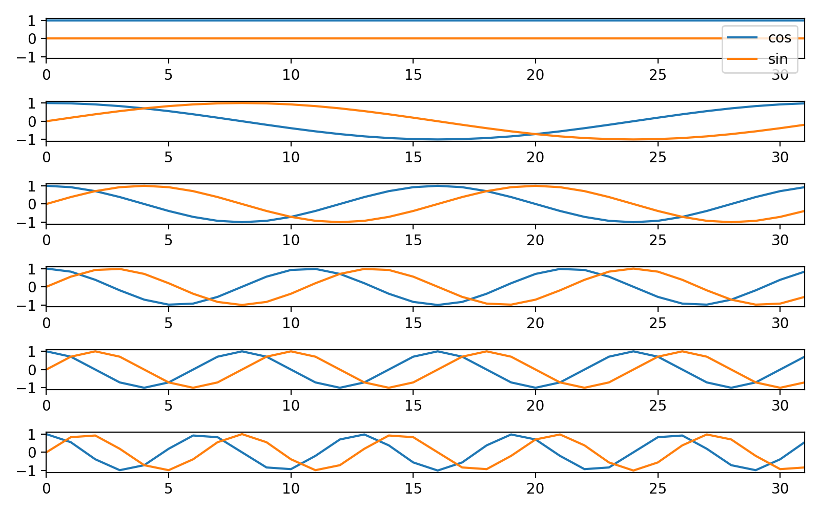
Here are some plots of \(\vec{c_k}\), \(\vec{s_k}\) for \(k \in 0, 1, 2, 3, 4, 5\):

>>> fig, axes = plt.subplots(6, 1, figsize=(8, 5))
>>> ns = np.arange(N)
>>> one_cycle = 2 * np.pi * ns / N
>>> for k in range(6):
...     t_k = k * one_cycle
...     axes[k].plot(ns, np.cos(t_k), label='cos')
...     axes[k].plot(ns, np.sin(t_k), label='sin')
...     axes[k].set_xlim(0, N-1)
...     axes[k].set_ylim(-1.1, 1.1)
[...)
>>> axes[0].legend()
<...>
>>> plt.tight_layout()

(png, hires.png, pdf)

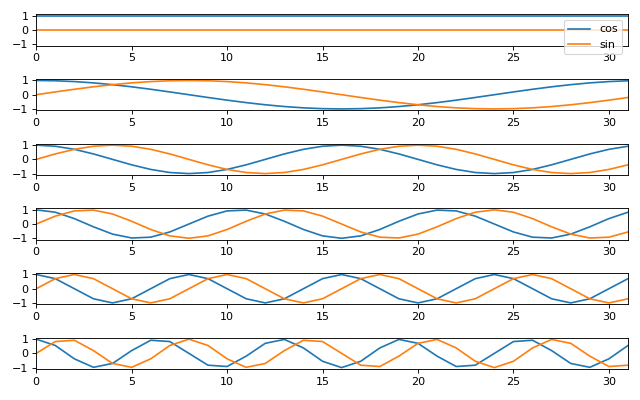
To rephrase: \(\vec{c_k}, \vec{s_k}\) are cosine / sine waves with \(k\) cycles over the \(N\) indices.

So, the \(X_k\) value is the dot product of the \(\vec{x}\) with a cosine wave of \(k\) cycles minus \(i\) times the dot product of \(\vec{x}\) with the sine wave of \(k\) cycles.

While this is all fresh in our minds, let us fill out the equivalent notation for the inverse transform.

\[\begin{split}\vec{t_n} \triangleq \left[ n 2 \pi \frac{k}{N} \;\mathrm{for}\; k \in =0,1,\ldots,N-1 \right] \\ \vec{c_n} \triangleq \left[ \cos(t_{n,k}) \;\mathrm{for}\; k \in 0,1,\ldots,N-1 \right] \\ \vec{s_n} \triangleq \left[ \sin(t_{n,k}) \;\mathrm{for}\; k \in 0,1,\ldots,N-1 \right]\end{split}\]

Because both \(n\) and \(k\) have indices from \(0 .. N-1\):

\[\begin{split}\vec{t_k} = \vec{t_n} \;\mathrm{where}\; k=n \\ \vec{c_k} = \vec{c_n} \;\mathrm{where}\; k=n \\ \vec{s_k} = \vec{s_n} \;\mathrm{where}\; k=n\end{split}\]

We will return to this point fairly soon.

The inverse transform is now:

\[x_n = \frac{1}{N} \vec{X} \cdot \vec{c_n} + i \frac{1}{N} \vec{X} \cdot \vec{s_n}\]

Rewriting the DFT with cosine and sine basis matrices

Instead of writing the formulae for the individual elements \(X_k\) and \(x_n\), we can use matrices to express our formulae in terms of the vectors \(\vec{X}, \vec{x}\).

\(\newcommand{C}{\mathbf{C}} \newcommand{S}{\mathbf{S}}\) Define a matrix \(\C\) that has rows \([\vec{c_0}, \vec{c_1}, ..., \vec{c_{N-1}}]\):

\[\begin{split}\C \triangleq \begin{bmatrix} c_{0,0}, c_{0, 1}, ..., c_{0, N-1} \\ c_{1,0}, c_{1, 1}, ..., c_{1, N-1} \\ ... \\ c_{N-1,0}, c_{N-1, 1}, ..., c_{N-1, N-1} \\ \end{bmatrix}\end{split}\]

Call \(\C\) the cosine basis matrix.

Define a matrix \(\S\) that has rows \([\vec{s_0}, \vec{s_1}, ..., \vec{s_{N-1}}]\):

\[\begin{split}\S \triangleq \begin{bmatrix} s_{0,0}, s_{0, 1}, ..., s_{0, N-1} \\ s_{1,0}, s_{1, 1}, ..., s_{1, N-1} \\ ... \\ s_{N-1,0}, s_{N-1, 1}, ..., s_{N-1, N-1} \\ \end{bmatrix}\end{split}\]

Call \(\S\) the sine basis matrix.

Now we can rewrite the forward and inverse DFT as matrix products:

\[\begin{split}\vec{X} = \C \cdot \vec{x} - i \S \cdot \vec{x} \\ \vec{x} = \frac{1}{N} \C \cdot \vec{X} + i \frac{1}{N} \S \cdot \vec{X}\end{split}\]

This gives us the same calculation for \(X_k\) and \(x_n\) as we have above using the vector dot products. Write row \(k\) of \(\C\) as \(C_{k,:}\). Row \(k\) of \(\S\) is \(S_{k,:}\). Thus, from the rules of matrix multiplication:

\[\begin{split}X_k = C_{k,:} \cdot \vec{x} - i S_{k,:} \cdot \vec{x} \\ = \vec{x} \cdot \vec{c_k} - i \vec{x} \cdot \vec{s_k}\end{split}\]

and (inverse transform):

\[\begin{split}x_n = \frac{1}{N} C_{n,:} \cdot \vec{X} + i \frac{1}{N} S_{n,:} \cdot \vec{X} \\ = \frac{1}{N} \vec{X} \cdot \vec{c_n} + i \frac{1}{N} \vec{X} \cdot \vec{s_n}\end{split}\]

We can build \(\C\) and \(\S\) for our case with \(N=32\):

>>> C = np.zeros((N, N))
>>> S = np.zeros((N, N))
>>> ns = np.arange(N)
>>> one_cycle = 2 * np.pi * ns / N
>>> for k in range(N):
...     t_k = k * one_cycle
...     C[k, :] = np.cos(t_k)
...     S[k, :] = np.sin(t_k)

We get the same result using this matrix formula, as we do using the canned DFT:

>>> # Recalculate the forward transform with C and S
>>> X_again = C.dot(x) - 1j * S.dot(x)
>>> assert np.allclose(X, X_again)  # same result as for np.fft.fft
>>> # Recalculate the inverse transform
>>> x_again = 1. / N * C.dot(X) + 1j / N * S.dot(X)
>>> assert np.allclose(x, x_again)  # as for np.fft.ifft, we get x back

Displaying the DFT transform

We can show the matrix calculation of the DFT as images. To do this we will use some specialized code. If you are running this tutorial yourself, download dft_plots.py to the directory containing this page.

>>> # Import the custom DFT plotting code
>>> import dft_plots as dftp

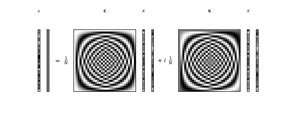
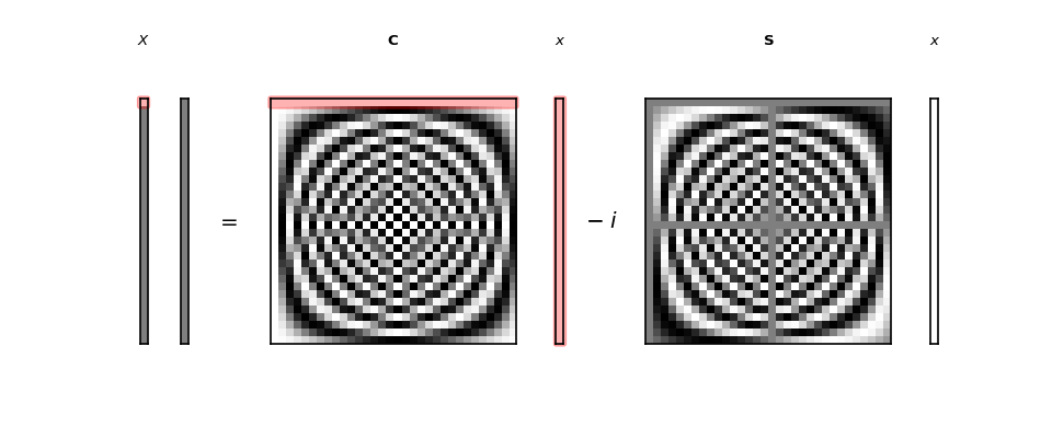
Here we show the forward DFT given by the formula:

\[\vec{X} = \C \cdot \vec{x} - i \S \cdot \vec{x}\]

>>> # Show image sketch for forward DFT
>>> sketch = dftp.DFTSketch(x)
>>> sketch.sketch(figsize=(12, 5))

(png, hires.png, pdf)

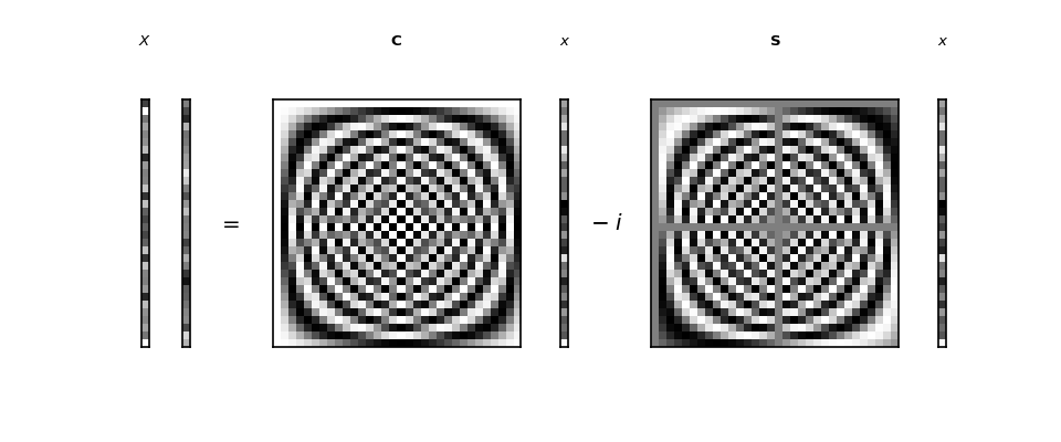
The plot shows each matrix and vector as grayscale, where mid gray corresponds to 0, black corresponds to the most negative value and white to the most positive value. For example the first four values in the vector \(\vec{x}\) are:

>>> x[:4]
array([ 0.4967, -0.1383,  0.6477,  1.523 ])

You can see \(\vec{x}\) shown at the right of the graphic as a column vector. The grayscale of the top four values in the graphic are light gray, mid gray, light gray, and near white, corresponding to the values above.

\(\vec{X}\) is a vector of complex numbers.

On the left of the equals sign you see the complex vector \(\vec{X}\) displayed as two columns.

Define \(\R{\vec{X}}\) to be the vector containing the real parts of the complex values in \(\vec{X}\). Define \(\I{\vec{X}}\) to be the vector containing the imaginary parts of \(\vec{X}\):

\[\begin{split}\R{\vec{X}} \triangleq [\R{X_0}, \R{X_1}, ..., \R{X_{N-1}}] \\ \I{\vec{X}} \triangleq [\I{X_0}, \I{X_1}, ..., \I{X_{N-1}}]\end{split}\]

The left hand column in the graphic shows \(\R{\vec{X}}\), and the column to the right of that shows \(\I{\vec{X}}\).

To the right of the equals sign we see the representation of \(\C \cdot \vec{x}\) and \(\S \cdot \vec{x}\), with \(\vec{x}\) displayed as a column vector.

\(\C\) and \(\S\) have some interesting patterns which we will explore in the next section.

We can show the inverse DFT in the same way:

\[\vec{x} = \frac{1}{N} \C \cdot \vec{X} + i \frac{1}{N} \S \cdot \vec{X}\]

>>> sketch.sketch(inverse=True, figsize=(12, 5))

(png, hires.png, pdf)

The output from the inverse transform is a complex vector, but in our case, where the input to the DFT was a vector of real numbers, the imaginary parts are all zero, and the real part is equal to our input to the forward DFT : \(\vec{x}\). We will see why the imaginary parts are all zero in the following sections.

Real and complex input to the DFT

This page is mostly concerned with the common case where the input to the forward DFT is a vector of real numbers. The mathematics also works for the case where the input to the forward DFT is a vector of complex numbers:

>>> complex_x = np.array(  # A Random array of complex numbers
...       [ 0.61-0.83j, -0.82-0.12j, -0.50+1.14j,  2.37+1.67j,  1.62+0.69j,
...         1.61-0.06j,  0.54-0.73j,  0.89-1.j  ,  0.17-0.71j,  0.75-0.01j,
...        -1.06-0.14j, -2.53-0.33j,  1.74+0.83j,  1.34-0.64j,  1.47+0.71j,
...         0.82+0.4j , -1.59-0.58j,  0.13-1.02j,  0.47-0.73j,  1.45+1.31j,
...         1.32-0.28j,  1.58-2.13j,  0.75-0.43j,  1.24+0.4j ,  0.02+1.08j,
...         0.07-0.57j, -1.21+1.08j,  1.38+0.54j, -1.35+0.3j , -0.61+1.08j,
...        -0.96+1.81j, -1.95+1.64j])
>>> complex_X = np.fft.fft(complex_x)  # Canned DFT
>>> complex_X_again = C.dot(complex_x) - 1j * S.dot(complex_x)  # Our DFT
>>> # We get the same result as the canned DFT
>>> assert np.allclose(complex_X, complex_X_again)

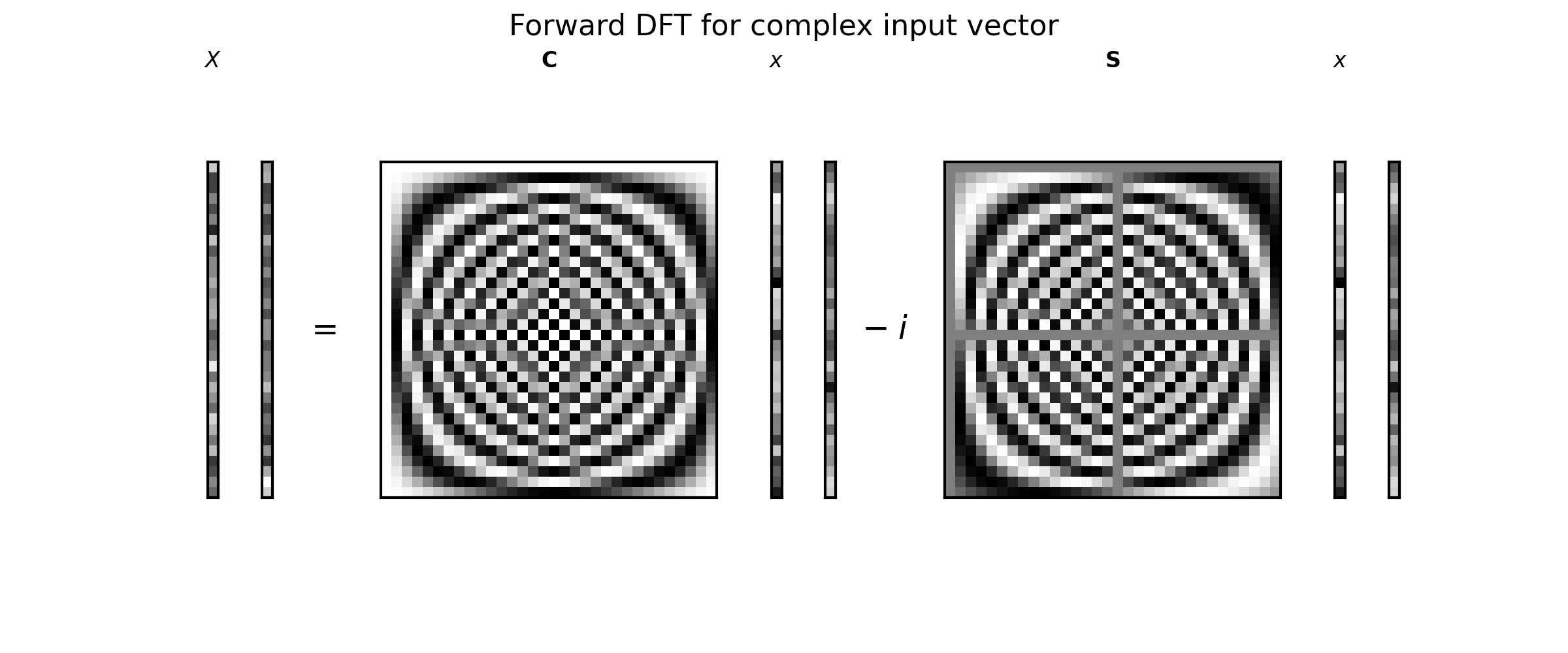
The sketch of the complex forward DFT looks like this:

>>> sketch = dftp.DFTSketch(complex_x)
>>> sketch.sketch(figsize=(12, 5))
>>> sketch.title('Forward DFT for complex input vector')

(png, hires.png, pdf)

The input \(\vec{x}\) vectors following \(\C\) and \(\S\) are now complex, with a real and a complex column for the real and complex vectors in \(\vec{x}\).

For what follows, unless we say otherwise, we will always be talking about real number input to the DFT.

Some properties of the cosine and sine basis matrices

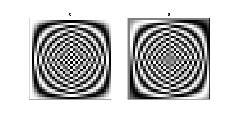
First we note that \(\C\) and \(\S\) are always real matrices, regardless of the input \(\vec{x}\) or \(\vec{X}\).

Let’s show \(\C\) and \(\S\) as grayscale images again:

>>> fig, axes = plt.subplots(1, 2, figsize=(10, 5))
>>> dftp.show_array(axes[0], dftp.scale_array(C))
>>> axes[0].set_title("$\mathbf{C}$")
<...>
>>> dftp.show_array(axes[1], dftp.scale_array(S))
>>> axes[1].set_title("$\mathbf{S}$")
<...>

(png, hires.png, pdf)

Mirror symmetry

From the images we see that the bottom half of \(\C\) looks like a mirror image of the top half of \(\C\). The bottom half of \(\S\) looks like a sign flipped (black \(\Leftrightarrow\) white) mirror image of the top half of \(\S\). In fact this is correct:

\[\begin{split}C_{p,:} = C_{N-p,:} \; \mathrm{for} \; p > 0 \\ S_{p,:} = -S_{N-p,:} \; \mathrm{for} \; p > 0\end{split}\]

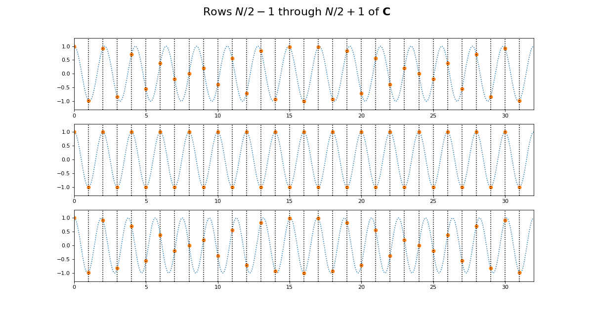
Why is this? Let’s look at lines from the center of \(\C\). Here we are plotting the continuous cosine function with dotted lines, with filled circles to represent the discrete samples we took to fill the row of \(\C\):

>>> center_rows = [N / 2. - 1, N / 2., N / 2. + 1]
>>> fig = dftp.plot_cs_rows('C', N, center_rows)
>>> fig.suptitle('Rows $N / 2 - 1$ through $N / 2 + 1$ of $\mathbf{C}$',
...              fontsize=20)
<...>

(png, hires.png, pdf)

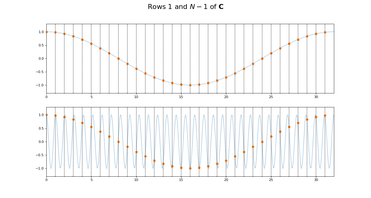
The first plot in this grid is for row \(k = N / 2 - 1\). This row starts sampling just before the peak and trough of the cosine. In the center is row \(k = N / 2\) of \(\C\). This is sampling the cosine wave exactly at the peak and trough. When we get to next row, at \(k = N / 2 + 1\), we start sampling after the peak and trough of the cosine, and these samples are identical to the samples just before the peak and trough, at row \(k = N / 2 - 1\). Row \(k = N / 2\) is sampling at the Nyquist sampling frequency, and row \(k = N / 2 + 1\) is sampling at a frequency lower than Nyquist and therefore it is being aliased to the same apparent frequency as row \(k = N / 2 - 1\).

This might be more obvious plotting rows 1 and N-1 of \(\C\):

>>> fig = dftp.plot_cs_rows('C', N, [1, N-1])
>>> fig.suptitle('Rows $1$ and $N - 1$ of $\mathbf{C}$',
...              fontsize=20)
<...>

(png, hires.png, pdf)

Of course we get the same kind of effect for \(\S\):

>>> fig = dftp.plot_cs_rows('S', N, center_rows)
>>> fig.suptitle('Rows $N / 2 - 1$ through $N / 2 + 1$ of $\mathbf{S}$',
...              fontsize=20)
<...>

(png, hires.png, pdf)

>>> fig = dftp.plot_cs_rows('S', N, [1, N-1])
>>> fig.suptitle('Rows $1$ and $N - 1$ of $\mathbf{S}$',
...              fontsize=20)
<...>

(png, hires.png, pdf)

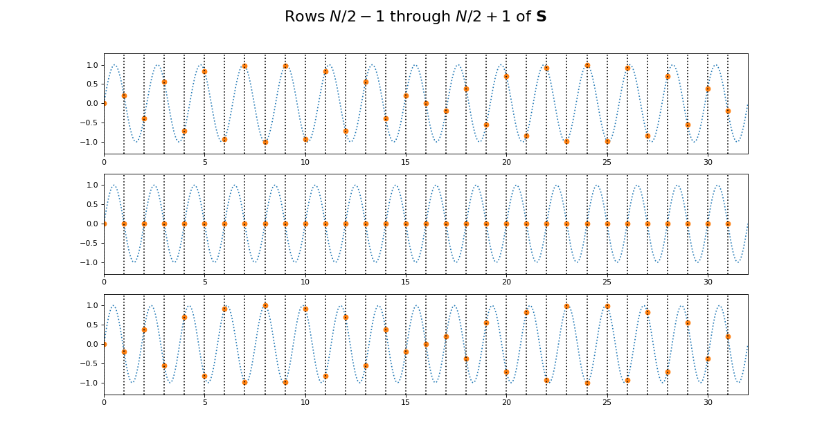
Notice that for \(\S\), the sine waves after \(k = N / 2\) are sign-flipped relative to their matching rows before \(k = N / 2\). Thus row \(k = N / 2 + 1\) will be aliased to the same frequency as for row \(k = N / 2 - 1\), but with a negative sign.

It is this sign-flip that leads to the concept of negative frequency in the DFT, and to the property of conjugate symmetry from the DFT on a vector of real numbers. We will hear more about these later.

Matrix symmetry

The next thing we notice about \(\C\) and \(\S\) is that they are transpose symmetric matrices:

\[\begin{split}\C = \C^T \\ \S = \S^T \\\end{split}\]

>>> assert np.allclose(C, C.T)
>>> assert np.allclose(S, S.T)

Why is this? Consider the first column of \(\C\). This is given by \(\cos(k 2 \pi 0 / N) = \cos(0)\), and thus, like the first row of \(\C\), is always = 1.

Now consider the second row of \(\C\). This is a cosine sampled at horizontal axis values:

\[\vec{t_1} \triangleq \left[ 2 \pi \frac{n}{N} \;\mathrm{for}\; n \in 0,1,\ldots,N-1 \right]\]

Call \(t_{k, n}\) the value of \(\vec{t_k}\) at index \(n\). Now consider the second column of \(\C\). This is a cosine sampled at horizontal axis values for \(n = 1\):

\[\begin{split}t_{0,1} = (0) 2 \pi \frac{1}{N} \\ t_{1,1} = (1) 2 \pi \frac{1}{N} \\ ... \\ t_{N-1,1} = (N-1) 2 \pi \frac{1}{N} \\\end{split}\]

In general, because the sequence \(k 0,1,,N-1 \) is equal to the sequence \(n \in 0,1,\ldots,N-1\), this means that the column sampling positions for row \(n \in t_{0, n}, t_{1, n}, ... , t_{N-1, n}\) are equal to the row sampling positions for corresponding (\(k = n\)) row \(k \in t_{k, 0}, t_{k, 1}, ... , t_{k, N-1}\). Write column \(z\) of \(\C\) as \(C_{:,z}\); column \(z\) of \(\S\) is \(S_{:, z}\). Therefore \(C_{z, :} = C_{:, z}, S_{z, :} = S_{:, z}\).

Row dot products and lengths

It is useful to look at the dot products of the rows of \(\C\) and \(\S\). The dot product of each row with itself gives the squared length of the vector in that row.

The vector length of a vector \(\vec{v}\) with \(N\) elements is written as \(\| \vec{v} \|\), and defined as:

\[\| \vec{v} \| \triangleq \sqrt{\sum_{n=0}^{N-1} v_n^2} = \sqrt{ \vec{v} \cdot \vec{v} }\]

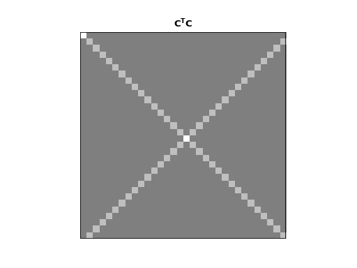
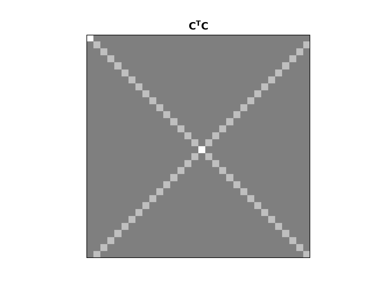
The dot products of different rows of \(\C\) and \(\S\) give an index of the strength of the relationship between the rows. We can look at the dot products of all the rows of \(\C\) with all other rows with the matrix multiplication \(\C^T \C\):

>>> dftp.show_array(plt.gca(), dftp.scale_array(C.T.dot(C)))
>>> plt.title("$\mathbf{C^TC}$")
<...>

(png, hires.png, pdf)

The image shows us that the dot product between the rows of \(\C\) is 0 everywhere except:

• the dot products of the rows with themselves (the squared vector lengths);
• the dot products of the mirror image vectors such as \(\vec{c_1}\) and \(\vec{c_{N-1}}\). Because \(\vec{c_n} = \vec{c_{N-n}}\), these dot products are the same as the \(\| \vec{c_n} \|^2\).

The squared row lengths are:

>>> np.diag(C.T.dot(C))
array([ 32.,  16.,  16.,  16.,  16.,  16.,  16.,  16.,  16.,  16.,  16.,
        16.,  16.,  16.,  16.,  16.,  32.,  16.,  16.,  16.,  16.,  16.,
        16.,  16.,  16.,  16.,  16.,  16.,  16.,  16.,  16.,  16.])

Notice that the rows \(\vec{c_0}\) and \(\vec{c_{N / 2}}\) have squared length \(N\), and the other rows have squared length \(N / 2\).

We can do the same for \(\S\):

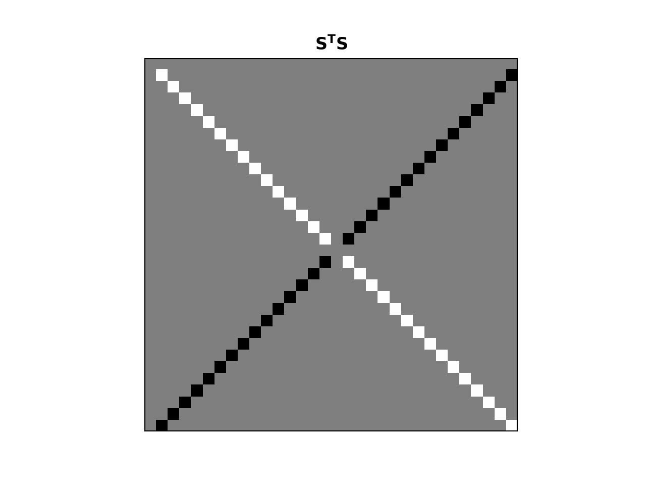
>>> dftp.show_array(plt.gca(), dftp.scale_array(S.T.dot(S)))
>>> plt.title("$\mathbf{S^TS}$")
<...>

(png, hires.png, pdf)

Remember that \(\vec{s_0}\) and \(\vec{s_{n/2}}\) are all 0 vectors. The dot product of these rows with any other row, including themselves, is 0. All other entries in this \(\S^T \S\) matrix are zero except:

• the dot products of rows with themselves (other than \(\vec{s_0}\) and \(\vec{s_{n/2}}\));
• the dot products of the flipped mirror image vectors such as \(\vec{s_1}\) and \(\vec{s_{N-1}}\). Because \(\vec{s_n} = -\vec{s_{N-n}}\), these dot products are the same as \(-\| \vec{s_n} \|^2\).

The squared row lengths are:

>>> np.diag(S.T.dot(S))
array([  0.,  16.,  16.,  16.,  16.,  16.,  16.,  16.,  16.,  16.,  16.,
        16.,  16.,  16.,  16.,  16.,   0.,  16.,  16.,  16.,  16.,  16.,
        16.,  16.,  16.,  16.,  16.,  16.,  16.,  16.,  16.,  16.])

The rows \(\vec{s_0}\) and \(\vec{s_{N / 2}}\) have squared length \(0\), and the other rows have squared length \(N / 2\).

Finally, let’s look at the relationship between the rows of \(\C\) and the rows of \(\S\):

>>> np.allclose(C.T.dot(S), 0)
True

The rows of \(\C\) and \(\S\) are completely orthogonal.

In fact these relationships hold for \(\C\) and \(\S\) for any \(N\).

Proof for \(\C, \S\) dot products

We can show these relationships with some more or less basic trigonometry.

Let’s start by looking at the dot product of two rows from \(\C\). We will take rows \(\vec{c_p} =\C_{p,:}\) and \(\vec{c_q} = \C_{q,:}\). As we remember, these vectors are:

\[\begin{split}\vec{c_p} = \left[ \cos(p n \frac{2 \pi}{N}) \;\mathrm{for}\; n \in 0,1,\ldots,N-1 \right] \\ \vec{c_q} = \left[ \cos(q n \frac{2 \pi}{N}) \;\mathrm{for}\; n \in 0,1,\ldots,N-1 \right]\end{split}\]

So:

\[\vec{c_p} \cdot \vec{c_q} = \sum_{n=0}^{N-1} \cos(p n \frac{2 \pi}{N}) \cos(q n \frac{2 \pi}{N})\]

Our trigonometry tells us that:

\[\cos \alpha \cos \beta = \frac{1}{2} [ \cos(\alpha + \beta) - \cos(\alpha - \beta) ]\]

We can rewrite the dot product as the addition of two sums of cosines:

\[\vec{c_p} \cdot \vec{c_q} = \frac{1}{2} \sum_{n=0}^{N-1} \cos((p + q) n \frac{2 \pi}{N}) + \frac{1}{2} \sum_{n=0}^{N-1} \cos((p - q) n \frac{2 \pi}{N})\]

Now we can use the formulae for sums of arithmetic progressions of cosines and sines to solve these equations. Here are the formulae:

\[\begin{split}R \triangleq \frac{\sin(N \frac{1}{2}d)}{\sin(\frac{1}{2} d)} \\ \sum_{n=0}^{N-1} \cos(a + nd) = \begin{cases} N \cos a & \text{if } \sin(\frac{1}{2}d) = 0 \\ R \cos ( a + (N - 1) \frac{1}{2} d) & \text{otherwise} \end{cases} \\ \sum_{n=0}^{N-1} \sin(a + nd) = \begin{cases} N \sin a & \text{if } \sin(\frac{1}{2}d) = 0 \\ R \sin ( a + (N - 1) \frac{1}{2} d) & \text{otherwise} \end{cases}\end{split}\]

For our \(\C, \S\) row dot product sums, starting angle \(a\) is always 0, and the \(d\) value in the formulae are always integer multiples of \(\frac{2 \pi}{N}\). For example, \(d = (p \pm q) \frac{2 \pi}{N}\) in the equations above. For our case, we can write \(d = g \frac{2 \pi}{N}\) where \(g\) is an integer.

\[\begin{split}R = \frac{ \sin( g N \frac{1}{2} \frac{2 \pi}{N} ) } { \sin( g \frac{1}{2} \frac{2 \pi}{N} ) } \\ = \frac{ \sin( g \pi ) } { \sin( \frac{g}{N} \pi ) }\end{split}\]

Because \(g\) is an integer, the numerator of \(R\) will always be 0, so the resulting sum is zero unless the denominator of \(R\) is zero. The denominator is zero only if \(g\) is a multiple of N, including 0. When the denominator is zero, the sum will be equal to \(N \cos(a) = N \cos(0) = N\) for a cosine series or \(N \sin(a) = N \sin(0) = 0\) for a sine series.

Now we can calculate our dot product:

\[\begin{split}\vec{c_p} \cdot \vec{c_q} = \begin{cases} \frac{1}{2} N + \frac{1}{2} N = N & \text{if } p = q, p \in 0, N/2 \\ \frac{1}{2} N & \text{if } p = q, p \notin 0, N/2 \\ \frac{1}{2} N & \text{if } p + q = N, p \ne N/2 \\ 0 & \text{otherwise} \end{cases}\end{split}\]

We can apply the same kind of logic to the rows of \(\S\):

\[\sin \alpha \sin \beta = \frac{1}{2} [ \cos(\alpha - \beta) - \cos(\alpha + \beta) ]\]

So:

\[\vec{s_p} \cdot \vec{s_q} = \frac{1}{2} \sum_{n=0}^{N-1} \cos((p - q) n \frac{2 \pi}{N}) - \frac{1}{2} \sum_{n=0}^{N-1} \cos((p + q) n \frac{2 \pi}{N})\]

This gives:

\[\begin{split}\vec{s_p} \cdot \vec{s_q} = \begin{cases} 0 & \text{if } p = q, p \in 0, N/2 \\ \frac{1}{2} N & \text{if } p = q, p \notin 0, N/2 \\ -\frac{1}{2} N & \text{if } p + q = N, p \ne N/2 \\ 0 & \text{otherwise} \end{cases}\end{split}\]

Introducing vector projection

If you are not familiar with projection, I highly recommend the tutorials over at Khan academy.

If you know projection, you may think of a dot product like \(\vec{x} \cdot \vec{c_k}\) as part of the projection of our input signal \(\vec{x}\) onto the cosine vector \(\vec{c_k}\).

Projection involves calculating the amount of a particular signal vector (such as a cosine wave) in another signal vector (such as our input data \(\vec{x}\)).

The Pearson product-moment correlation coefficient uses the dot product to test for relationship between two variables. In our case, except for the first cosine vector \(\vec{c_0} = \vec{1}\), the dot products \(\vec{x} \cdot \vec{c_k}\) and \(\vec{x} \cdot \vec{s_k}\) are proportional to the Pearson product-moment correlation coefficient between \(\vec{c_k}\) and \(\vec{x}\) or \(\vec{s_k}\) and \(\vec{x}\), respectively.

The projection of a vector \(\vec{a}\) onto a vector \(\vec{b}\) is given by:

\[proj_{\vec{b}}\vec{a} \triangleq g \vec{b}\]

where \(g\) is a scalar that we will call the projection coefficient:

\[g = \frac{\vec{a} \cdot \vec{b}}{\vec{b} \cdot \vec{b}}\]

Note that \(\vec{b} \cdot \vec{b}\) is also \(\| \vec{b} \|^2\), so we can also write:

\[g = \frac{\vec{a} \cdot \vec{b}}{\| \vec{b} \|^2}\]

The result of the projection \(proj_{\vec{b}}\vec{a}\) is a copy of \(\vec{b}\) scaled by \(g\) - the scalar amount of \(\vec{a}\) present in \(\vec{b}\).

Forward and inverse DFT as vector projection

Projection and the DFT

The principle of the DFT on real input is the following.

In the forward transform:

• We calculate the data we need to form the projection coefficients for projecting the input data onto the cosines and sine waves in the rows of \(\C\) and \(\S\).
• The projection data for the cosines goes into the real part of \(\vec{X}\) : \(\R{\vec{X}}\). The projection data for the sines goes into the imaginary part \(\I{\vec{X}}\);

In the inverse transform:

• We complete the calculation of the projection coefficients \(g\) for each cosine and sine wave in \(\C, \S\);
• We use the projection coefficients to project the original data \(\vec{X}\) onto the set of cosines and sines in \(\C\), \(\S\). Each projection forms a new output vector, to give projection vectors \([proj_{\vec{c_0}} \vec{x}, proj_{\vec{c_1}} \vec{x}, ..., proj_{\vec{s_0}} \vec{x}, proj_{\vec{s_1}} \vec{x}, ...]\);
• We sum up all the projection vectors to reconstruct the original data \(\vec{X}\).

This is how it works in principle. There are some complications to the way it works in practice, due to the generality of the DFT in accepting real and complex input. In the next sections we will go through some examples to show how the forward and inverse transform work in detail.

>>> # Does it actually work?
>>> unique_Cs = C[:N//2+1, :]
>>> unique_Ss = S[1:N//2, :]
>>> small_n = len(unique_Ss)
>>> cos_dots = unique_Cs.dot(x)
>>> sin_dots = unique_Ss.dot(x)
>>> cos_gs = cos_dots / ([N] + [N//2] * small_n + [N])
>>> sin_gs = sin_dots / ([N//2] * small_n)
>>> cos_projections = cos_gs[:, None] * unique_Cs
>>> sin_projections = sin_gs[:, None] * unique_Ss
>>> x_back = np.sum(np.vstack((cos_projections, sin_projections)), axis=0)
>>> x_back - x
array([-0.,  0., -0.,  0., -0., -0.,  0., -0.,  0., -0.,  0., -0.,  0.,
       -0., -0.,  0., -0.,  0., -0., -0.,  0.,  0., -0., -0.,  0., -0.,
        0.,  0.,  0., -0.,  0., -0.])

The first element in \(\vec{X}\) for real input

From our matrix multiplication, we know the first element of \(\vec{X}\) comes from:

\[X_0 = C_{0, :} \cdot \vec{x} - i S_{0, :} \cdot \vec{x} = \vec{c_0} \cdot \vec{x} - i \vec{s_0} \cdot \vec{x}\]

We can represent this by highlighting the relevant parts of the matrix multiplication:

We can simplify further because we know what \(\vec{c_0}\) and \(\vec{s_0}\) are:

\[X_0 = \vec{1} \cdot \vec{x} - i \vec{0} \cdot \vec{x} = \vec{1} \cdot \vec{x}\]

This final dot product can also be written as:

\[X_0 = \sum_{n=0}^{N-1}{x_n}\]

That is, \(X_0\) is a complex number with imaginary part = 0, where the real part contains the sum of the elements in \(\vec{x}\).

Is this true of our original input vector \(\vec{x}\)?

>>> print('Sum of x', np.sum(x))
Sum of x -4.3939
>>> print('First DFT coefficient X[0]', X[0])
First DFT coefficient X[0] (-4.3939+0j)

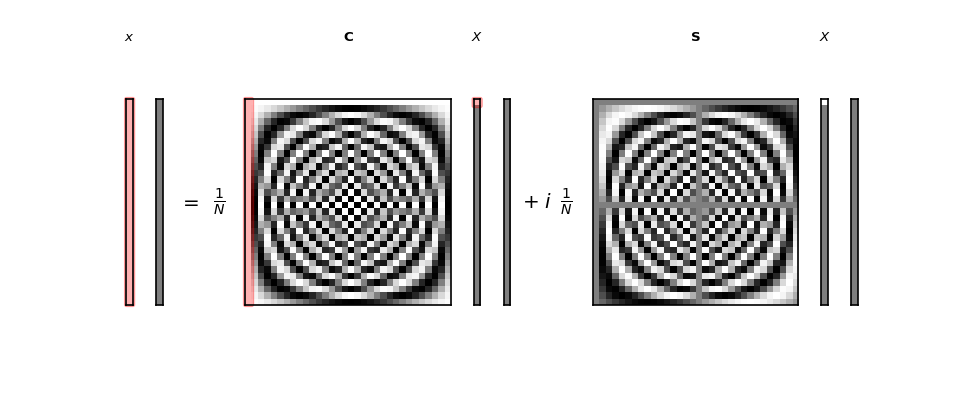
We can show how \(X_0\) comes about in the matrix multiplication by highlighting

• \(X_0\);
• the relevant row of \(\C\) : \(C_{0,:}\);
• the vector \(\vec{x}\).

We can leave out the relevant row of \(\S\) : \(S_{0,:}\) because it is all 0.

>>> sketch = dftp.DFTSketch(x)
>>> sketch.sketch(figsize=(12, 5))
>>> sketch.highlight('X_real', [0])
>>> sketch.highlight('C', [[0, ':']])
>>> sketch.highlight('x_c', [':'])

(png, hires.png, pdf)

DFT of a constant input vector

Next we will consider the forward and inverse DFT of an input vector that is constant.

Our input is vector with \(N\) elements, where every element = 2:

\[\vec{w} = [2, 2, ... 2]\]

We could also write \(\vec{w}\) as \(\vec{2}\).

>>> w = np.ones(N) * 2
>>> w
array([ 2.,  2.,  2.,  2.,  2.,  2.,  2.,  2.,  2.,  2.,  2.,  2.,  2.,
        2.,  2.,  2.,  2.,  2.,  2.,  2.,  2.,  2.,  2.,  2.,  2.,  2.,
        2.,  2.,  2.,  2.,  2.,  2.])

What DFT output \(\vec{W}\) will this generate?

We already know that \(W_0\) must be the sum of \(\vec{w}\):

>>> W = np.fft.fft(w)
>>> print('Sum of w', np.sum(w))
Sum of w 64.0
>>> print('First DFT coefficient W[0]', W[0])
First DFT coefficient W[0] (64+0j)

How about the rest of \(\vec{W}\)? All the remaining cosine and sine waves in \(\C, \S\) sum to zero over the rows (and columns):

>>> print('Sums over rows of C after first', np.sum(C[1:], axis=1))
Sums over rows of C after first [-0. -0. -0. -0. -0. -0.  0. -0.  0. -0. -0.  0. -0. -0. -0.  0. -0.  0.
 -0. -0.  0.  0. -0.  0. -0.  0.  0.  0.  0. -0.  0.]
>>> print('Sums over rows of S', np.sum(S, axis=1))
Sums over rows of S [ 0. -0. -0. -0.  0.  0.  0. -0.  0.  0.  0.  0.  0. -0. -0.  0. -0. -0.
  0. -0.  0.  0.  0.  0.  0. -0.  0.  0.  0. -0.  0.  0.]

For any vector \(\vec{v}\) that sums to zero, the dot product \(\vec{2} \cdot \vec{v}\) will be \(\sum_{n=0}^{N-1} 2 v_n = 2 \sum_{n=0}^{N-1} v_n = 0\).

So, we predict that all the rest of \(W_0\), real and imaginary, will be 0:

>>> W
array([ 64.+0.j,   0.+0.j,   0.+0.j,   0.+0.j,   0.+0.j,   0.+0.j,
         0.+0.j,   0.+0.j,   0.+0.j,   0.+0.j,   0.+0.j,   0.+0.j,
         0.+0.j,   0.+0.j,   0.+0.j,   0.+0.j,   0.+0.j,   0.+0.j,
         0.+0.j,   0.+0.j,   0.+0.j,   0.+0.j,   0.+0.j,   0.+0.j,
         0.+0.j,   0.+0.j,   0.+0.j,   0.+0.j,   0.+0.j,   0.+0.j,
         0.+0.j,   0.+0.j])

Let us show this in the matrix form:

>>> sketch = dftp.DFTSketch(w)
>>> sketch.sketch(figsize=(12, 5))
>>> sketch.highlight('X_real', [0])
>>> sketch.highlight('C', [[0, ':']])
>>> sketch.highlight('x_c', [':'])

(png, hires.png, pdf)

Cosines in the real part, sines in the imaginary part

The following only applies to real input to the DFT.

From the forward DFT formula on a vector of real numbers, we see that the \(\R{X}\) will contain the dot product of \(\vec{x}\) with the cosine basis, and \(\I{X}\) will contain the dot product of \(\vec{x}\) with the sine basis.

Imagine, for simplicity, that \(\vec{s_k} \cdot \vec{x} = 0\) for every \(k\), or (saying the same thing in a different way) \(\S \cdot \vec{x} = \vec{0}\).

In that case our forward DFT would be:

\[X = \C \cdot \vec{x}\]

and the inverse DFT would be:

\[X = \frac{1}{N} \C \cdot \vec{X}\]

In that case, \(\vec{X}\) would be a vector of real numbers, each expressing the amount of the corresponding cosine vector is present in the data.

We could then perfectly reconstruct our original data by summing up the result of projecting onto each cosine vector.

In the case of our constant input vector \(\vec{w}\), this is the case - there are no sine components in \(\vec{w}\) and \(\S \cdot \vec{x} = \vec{0}\).

So, \(\R{\vec{X}}\) contains all the information in \(\vec{w}\). In fact, as we have seen, \(\R{X_0}\) contains all the information in \(\vec{w}\).

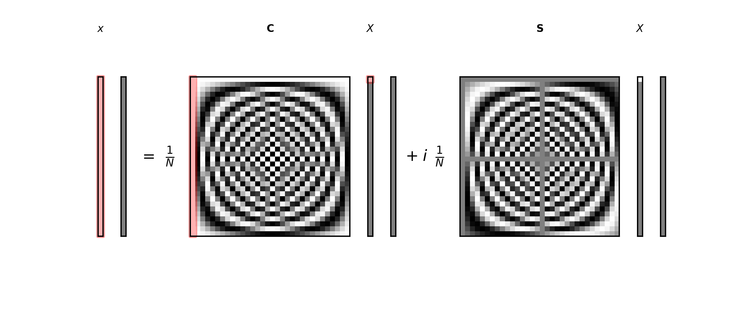
Rephrasing in terms of projection, \(W_0\) comes from \(\vec{1} \cdot \vec{w}\). This the top half of the \(g\) value for projecting the signal \(\vec{w}\) onto a vector of ones \(\vec{c_0}\) : \(g = \frac{\vec{w} \cdot \vec{1}}{\vec{1} \cdot \vec{1}}\). We know \(\vec{1} \cdot \vec{1} = N\) so the projection of \(\vec{w}\) onto \(\vec{1}\) is \(\frac{\vec{w} \cdot \vec{1}}{\vec{1} \cdot \vec{1}} \vec{1} = \frac{1}{N} \vec{w} \cdot \vec{1}\), and this is precisely what the inverse DFT will do:

\[\begin{split}w_0 = \frac{1}{N} \vec{1} \cdot \vec{W} - i \frac{1}{N} \vec{0} \cdot \vec{W} = \frac{1}{N} \vec{1} \cdot \vec{W} \\ w_1 = \frac{1}{N} \vec{1} \cdot \vec{W} \\ ... \\ w_{N-1} = \frac{1}{N} \vec{1} \cdot \vec{W}\end{split}\]

>>> w_again = np.zeros(w.shape, dtype=np.complex)
>>> c_0 = np.ones(N)
>>> for n in np.arange(N):
...     w_again[n] = 1. / N * c_0.dot(W)
>>> w_again
array([ 2.+0.j,  2.+0.j,  2.+0.j,  2.+0.j,  2.+0.j,  2.+0.j,  2.+0.j,
        2.+0.j,  2.+0.j,  2.+0.j,  2.+0.j,  2.+0.j,  2.+0.j,  2.+0.j,
        2.+0.j,  2.+0.j,  2.+0.j,  2.+0.j,  2.+0.j,  2.+0.j,  2.+0.j,
        2.+0.j,  2.+0.j,  2.+0.j,  2.+0.j,  2.+0.j,  2.+0.j,  2.+0.j,
        2.+0.j,  2.+0.j,  2.+0.j,  2.+0.j])

In matrix form:

>>> 1. / N * C.dot(W)
array([ 2.+0.j,  2.+0.j,  2.+0.j,  2.+0.j,  2.+0.j,  2.+0.j,  2.+0.j,
        2.+0.j,  2.+0.j,  2.+0.j,  2.+0.j,  2.+0.j,  2.+0.j,  2.+0.j,
        2.+0.j,  2.+0.j,  2.+0.j,  2.+0.j,  2.+0.j,  2.+0.j,  2.+0.j,
        2.+0.j,  2.+0.j,  2.+0.j,  2.+0.j,  2.+0.j,  2.+0.j,  2.+0.j,
        2.+0.j,  2.+0.j,  2.+0.j,  2.+0.j])

>>> sketch = dftp.DFTSketch(w)
>>> sketch.sketch(inverse=True, figsize=(12, 5))
>>> sketch.highlight('x_real', [':'])
>>> sketch.highlight('C', [[':', 0]])
>>> sketch.highlight('X_c_real', [0])

(png, hires.png, pdf)

DFT on a signal with a single cosine

Now let us look at the second coefficient, \(X_1\).

This was formed by dot products of the signal with cosine and sine waves having a single cycle across the whole signal:

\[\begin{split}\vec{t_1} \triangleq \left[ 2 \pi \frac{n}{N} \;\mathrm{for}\; n \in 0,1,\ldots,N-1 \right] \\ \vec{c_1} \triangleq \left[ \cos(t_{1,n}) \;\mathrm{for}\; n \in 0,1,\ldots,N-1 \right] \\ \vec{s_1} \triangleq \left[ \sin(t_{1,n}) \;\mathrm{for}\; n \in 0,1,\ldots,N-1 \right]\end{split}\]

Here are plots of \(\vec{c_1}, \vec{s_1}\):

>>> ns = np.arange(N)
>>> t_1 = 2 * np.pi * ns / N
>>> plt.plot(ns, np.cos(t_1), 'o:')
[...]
>>> plt.plot(ns, np.sin(t_1), 'o:')
[...]
>>> plt.xlim(0, N-1)
(...)
>>> plt.xlabel('n')
<...>

(png, hires.png, pdf)

If the input signal is a single cosine wave of amplitude 3, with one cycle over the signal, then we can predict \(X_1\). It will be the dot product of the input signal with \(c_1\), which is the same as \(3 c_1 \cdot c_1\):

>>> t_1 = 2 * np.pi * ns / N
>>> cos_x = 3 * np.cos(t_1)
>>> c_1 = np.cos(t_1)
>>> X = np.fft.fft(cos_x)
>>> print('First DFT coefficient for single cosine', to_4dp(X[1]))
First DFT coefficient for single cosine 48.0000-0.0000j
>>> print('Dot product of single cosine with c_1', cos_x.dot(c_1))
Dot product of single cosine with c_1 48.0
>>> print('3 * dot product of c_1 with itself', 3 * c_1.T.dot(c_1))
3 * dot product of c_1 with itself 48.0

Fitting all cosine phases with an added sine

Now it is time to bring the \(i \vec{x} \cdot \vec{s_k}\) part of the DFT into play.

By calculating the dot product of our input vector with a cosine wave of a given frequency, we detect any signal that matches that cosine with the given phase and the given frequency. In our example above, we used the DFT \(\vec{c_1}\) dot product to detect a cosine with phase offset 0 - the cosine starts at \(n = 0\).

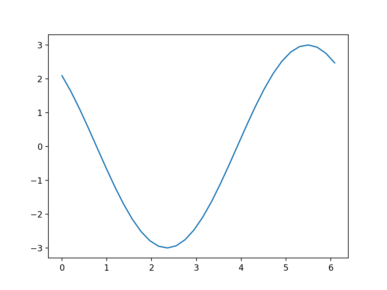
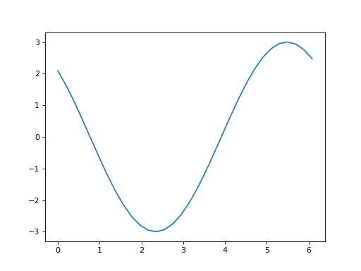
What happens if the cosine in the signal has a different phase? For example, what happens to the dot product if the cosine wave in our data is shifted by 0.8,

>>> cos_x_shifted = 3 * np.cos(t_1 + 0.8)
>>> plt.plot(t_1, cos_x_shifted)
[...]
>>> print('Dot product of shifted cosine with c_1',
...       to_4dp(cos_x_shifted.dot(c_1)))
Dot product of shifted cosine with c_1 33.4419

(png, hires.png, pdf)

When the cosine wave is shifted in our data, relative to the \(\vec{c_1}\), then the dot product of the signal against \(\vec{c_1}\) drops in value, and is therefore less successful at detecting this cosine wave.

This is the role of the \(\vec{s_k}\) vectors in the DFT. By calculating dot products with the \(\vec{s_k}\) vectors, we can detect cosine waves of any phase.

Let us see that in action first, and then explain why this is so.

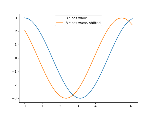
First, here is what happens to the dot products for the shifted and unshifted cosine waves:

>>> s_1 = np.sin(t_1)
>>> plt.plot(t_1, cos_x, label='3 * cos wave')
[...]
>>> plt.plot(t_1, cos_x_shifted, label='3 * cos wave, shifted')
[...]
>>> plt.legend()
<...>
>>> print('Dot product of unshifted cosine with c_1', cos_x.dot(c_1))
Dot product of unshifted cosine with c_1 48.0
>>> print('Dot product of unshifted cosine with s_1',
...       to_4dp(cos_x.dot(s_1)))
Dot product of unshifted cosine with s_1 -0.0000
>>> print('Dot product of shifted cosine with c_1',
...       to_4dp(cos_x_shifted.dot(c_1)))
Dot product of shifted cosine with c_1 33.4419
>>> print('Dot product of shifted cosine with s_1',
...       to_4dp(cos_x_shifted.dot(s_1)))
Dot product of shifted cosine with s_1 -34.4331

(png, hires.png, pdf)

Notice that the dot product with \(\vec{s_1}\) is effectively zero in the unshifted case, and goes up to around 34 in the shifted case.

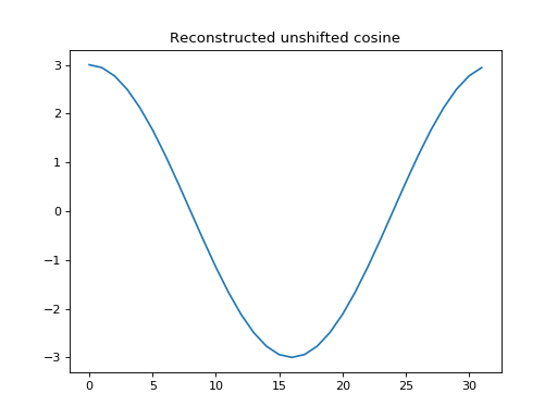
Now let us use the projections from these dot products to reconstruct the original vector (as we will soon do using the inverse DFT).

First we use the dot product with \(\vec{c_1}\) to reconstruct the unshifted cosine (the dot product with \(\vec{s_1}\) is zero, so we do not need it).

>>> # Reconstruct unshifted cos from dot product projection
>>> c_unshifted = cos_x.dot(c_1) / c_1.dot(c_1)
>>> proj_onto_c1 = c_unshifted * c_1
>>> plt.plot(ns, proj_onto_c1)
[...]
>>> plt.title('Reconstructed unshifted cosine')
<...>

(png, hires.png, pdf)

Now we can use the cosine and sine dot product to reconstruct the shifted cosine vector:

>>> # Reconstruct shifted cos from dot product projection
>>> c_cos_shifted = cos_x_shifted.dot(c_1) / c_1.dot(c_1)
>>> c_sin_shifted = cos_x_shifted.dot(s_1) / s_1.dot(s_1)
>>> proj_onto_c1 = c_cos_shifted * c_1
>>> proj_onto_s1 = c_sin_shifted * s_1
>>> reconstructed = proj_onto_c1 + proj_onto_s1
>>> plt.plot(ns, reconstructed)
[...]
>>> plt.title('Reconstructed shifted cosine')
<...>
>>> assert np.allclose(reconstructed, cos_x_shifted)

(png, hires.png, pdf)

The reason that this works for any phase shift is the angle sum rule.

The angle sum rule is:

\[\cos(\alpha \pm \beta) = \cos \alpha \cos \beta \mp \sin \alpha \sin \beta\]

To unpack the \(\pm, \mp\):

\[\begin{split}\cos(\alpha + \beta) = \cos \alpha \cos \beta - \sin \alpha \sin \beta \\ \cos(\alpha - \beta) = \cos \alpha \cos \beta + \sin \alpha \sin \beta\end{split}\]

See angle sum proof for a visual proof in the case of real angles \(\alpha, \beta\).

• Download this page as a Python code file;
• Download this page as a Jupyter notebook (no outputs).