\(\newcommand{L}[1]{\| #1 \|}\newcommand{VL}[1]{\L{ \vec{#1} }}\newcommand{R}[1]{\operatorname{Re}\,(#1)}\newcommand{I}[1]{\operatorname{Im}\, (#1)}\)

Correlated regressors

Written with J-B Poline.

Load and configure libraries:

>>> import numpy as np
>>> import numpy.linalg as npl
>>> import matplotlib.pyplot as plt
>>> # Make numpy print 4 significant digits for prettiness
>>> np.set_printoptions(precision=4, suppress=True)
>>> # Seed random number generator
>>> np.random.seed(42)

Hint

If running in the IPython console, consider running %matplotlib to enable interactive plots. If running in the Jupyter Notebook, use %matplotlib inline.

Imagine we have a TR (image) every 2 seconds, for 30 seconds. Here are the times of the TR onsets, in seconds:

>>> times = np.arange(0, 30, 2)
>>> times
array([ 0,  2,  4,  6,  8, 10, 12, 14, 16, 18, 20, 22, 24, 26, 28])

Now we make a function returning an HRF shape for an input vector of times:

>>> # Gamma distribution from scipy
>>> from scipy.stats import gamma

>>> def spm_hrf(times):
...     """ Return values for SPM-like HRF at given times """
...     # Make output vector
...     values = np.zeros(len(times))
...     # Only evaluate gamma above 0 (undefined at <= 0)
...     valid_times = times[times > 0]
...     # Gamma pdf for the peak
...     peak_values = gamma.pdf(valid_times, 6)
...     # Gamma pdf for the undershoot
...     undershoot_values = gamma.pdf(valid_times, 12)
...     # Combine them, put back into values vector
...     values[times > 0] = peak_values - 0.35 * undershoot_values
...     # Scale area under curve to 1
...     return values / np.sum(values)

Sample the HRF at the given times (to simulate an event starting at time 0), and at times - 2 (simulating an event starting at time 2):

>>> hrf1 = spm_hrf(times)
>>> hrf2 = spm_hrf(times - 2) # An HRF with 2 seconds (one TR) delay
>>> hrf1 = (hrf1 - hrf1.mean()) # Rescale and mean center
>>> hrf2 = (hrf2 - hrf2.mean())
>>> plt.plot(times, hrf1)
[...]
>>> plt.plot(times, hrf2)
[...]

(png, hires.png, pdf)

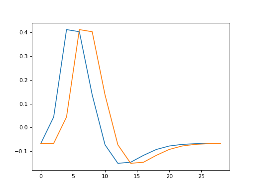
The Pearson correlation coefficient between the HRFs for the two events:

>>> np.corrcoef(hrf1, hrf2)
array([[ 1.    ,  0.7023],
       [ 0.7023,  1.    ]])

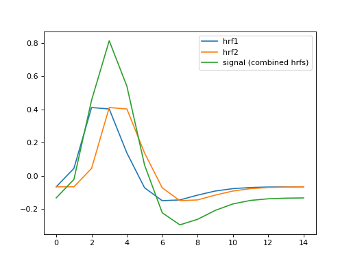
Make a signal that comes from the combination of the two HRFs:

>>> signal = hrf1 + hrf2
>>> plt.plot(hrf1, label='hrf1')
[...]
>>> plt.plot(hrf2, label='hrf2')
[...]
>>> plt.plot(signal, label='signal (combined hrfs)')
[...]
>>> plt.legend()
<...>

(png, hires.png, pdf)

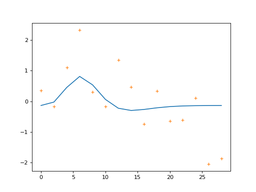
We’re going to make our simulated data from taking the signal (the two HRFs) and adding some random noise:

>>> noise = np.random.normal(size=times.shape)
>>> Y = signal + noise
>>> plt.plot(times, signal)
[...]
>>> plt.plot(times, Y, '+')
[...]

(png, hires.png, pdf)

We are going to model this simulated signal in several different ways. First, we make a model that only has the first HRF as a regressor (plus a column of ones to model the mean of the data):

>>> X_one = np.vstack((hrf1, np.ones_like(hrf1))).T
>>> plt.imshow(X_one, interpolation='nearest', cmap='gray')
<...>
>>> plt.title('Model with first HRF regressor only')
<...>

(png, hires.png, pdf)

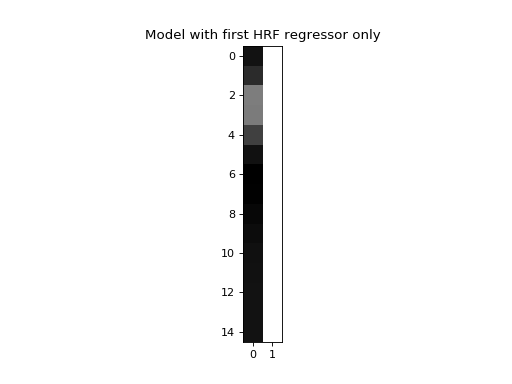
Next we make a model where we also include the second HRF as a regressor:

>>> X_both = np.vstack((hrf1, hrf2, np.ones_like(hrf1))).T
>>> plt.imshow(X_both, interpolation='nearest', cmap='gray')
<...>
>>> plt.title('Model with both HRF regressors')
<...>

(png, hires.png, pdf)

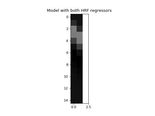
Now we make a very large number of data vectors, each with the signal (both HRFs) plus a different vector of noise.

>>> T = len(times)
>>> iters = 10000
>>> # Make 10000 Y vectors (new noise for each colum)
>>> noise_vectors = np.random.normal(size=(T, iters))
>>> # add signal to make data vectors
>>> Ys = noise_vectors + signal[:, np.newaxis]
>>> Ys.shape
(15, 10000)

We first fit the model with only the first HRF regressor to every (signal + noise) sample vector.

>>> # Fit X_one to signals + noise
>>> B_ones = npl.pinv(X_one).dot(Ys)

Next fit the model with both HRFs as regressors:

>>> # Fit X_both to signals + noise
>>> B_boths = npl.pinv(X_both).dot(Ys)

Remember that the students-t statistic is:

\[t = \frac{c^T \hat\beta}{\sqrt{\mathrm{var}(c^T \hat\beta)}}\]

which works out to:

\[t = \frac{c^T \hat\beta}{\sqrt{\hat{\sigma}^2 c^T (X^T X)^+ c}}\]

where \(\hat{\sigma}^2\) is our estimate of variance in the residuals, and \((X^T X)^+\) is the pseudo-inverse of \(X^T X\).

That’s the theory. So, what is the distribution of the estimates we get for the first beta, in the single-HRF model?

>>> plt.hist(B_ones[0], bins=50)
(...)
>>> print(np.std(B_ones[0]))
1.47669405469

(png, hires.png, pdf)

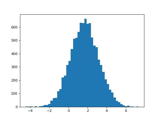
The standard deviation of the estimates is what we observe. Does this match what we would predict from the t-statistic formula above?

>>> C_one = np.array([1, 0])[:, None]  # column vector
>>> np.sqrt(C_one.T.dot(npl.pinv(X_one.T.dot(X_one)).dot(C_one)))
array([[ 1.485]])

Notice that the mean of the estimates, is somewhere above one, even though we only added 1 times the first HRF as the signal:

>>> print(np.mean(B_ones[0]))
1.68134012906

This is because the single first regresssor has to fit both the first HRF in the signal, and as much as possible of the second HRF in the signal, because there is nothing else in the model to fit the second HRF shape.

What estimates do we get for the first regressor, when we have both regressors in the model?

>>> plt.hist(B_boths[0], bins=50)
(...)
>>> print(np.mean(B_boths[0]), np.std(B_boths[0]))
0.968933589198 2.08274190893

(png, hires.png, pdf)

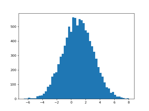
Two things have happened now we added the second (correlated) hrf2 regressor. First, the mean of the parameter for the hrf1 regressor has dropped to 1, because hrf1 is no longer having to model the signal from the second HRF. Second, the variability of the estimate has increased. This is what the bottom half of the t-statistic predicts:

>>> C_both = np.array([1, 0, 0])[:, None]  # column vector
>>> np.sqrt(C_both.T.dot(npl.pinv(X_both.T.dot(X_both)).dot(C_both)))
array([[ 2.0861]])

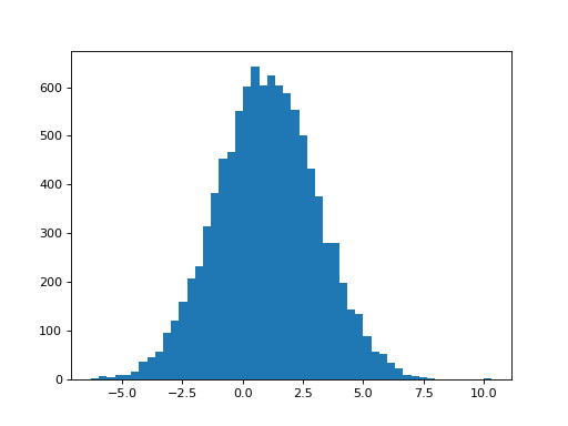
The estimate of the parameter for hrf2 has a mean of around 1, like the parameter estimates for hrf1. This is what we expect because we have 1 x hrf1 and 1 x hrf2 in the signal. Not surprisingly, the hrf2 parameter estimate has a similar variability to that for the hrf1 parameter estimate:

>>> plt.hist(B_boths[1], bins=50)
(...)
>>> print(np.mean(B_boths[1]), np.std(B_boths[1]))
1.01451944676 2.08038932821

(png, hires.png, pdf)

>>> C_both_1 = np.array([0, 1, 0])[:, None]  # column vector
>>> np.sqrt(C_both_1.T.dot(npl.pinv(X_both.T.dot(X_both)).dot(C_both_1)))
array([[ 2.0865]])

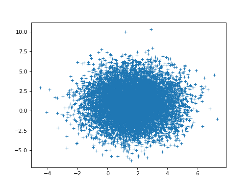
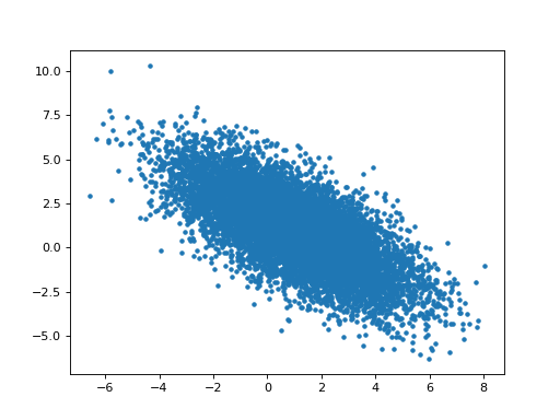
The parameter estimates for hrf1 and hrf2 are anti-correlated:

>>> # Relationship of estimated parameter of hrf1 and hrf2
>>> plt.plot(B_boths[0], B_boths[1], '.')
[...]
>>> np.corrcoef(B_boths[0], B_boths[1])
array([[ 1.    , -0.7052],
       [-0.7052,  1.    ]])

(png, hires.png, pdf)

Orthogonalizing hrf2 with respect to hrf1

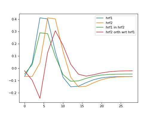
hrf2 is correlated with hrf1. That means that we can split up hrf2 into two vectors, one being a multiple of hrf1, and the other being the remaining unique contribution of hrf2. The sum of the two vectors is the original hrf2 regressor. Like this:

>>> # Regress hrf2 against hrf1 to get best fit of hrf2 using just hrf1
>>> y = hrf2
>>> X = hrf1[:, np.newaxis]  # hrf1 as column vector
>>> B_hrf1_in_hrf2 = npl.pinv(X).dot(y)  # scalar multiple of hrf1 to best fit hrf2
>>> hrf1_in_hrf2 = X.dot(B_hrf1_in_hrf2)  # portion of hrf2 that can be explained by hrf1
>>> unique_hrf2 = hrf2 - hrf1_in_hrf2  # portion of hrf2 that cannot be explained by hrf1
>>> plt.plot(times, hrf1, label='hrf1')
[...]
>>> plt.plot(times, hrf2, label='hrf2')
[...]
>>> plt.plot(times, hrf1_in_hrf2, label='hrf1 in hrf2')
[...]
>>> plt.plot(times, unique_hrf2, label='hrf2 orth wrt hrf1')
[...]
>>> plt.legend()
<...>
>>> # hrf1 part of hrf2, plus unique part, equals original hrf2
>>> np.allclose(hrf2, hrf1_in_hrf2 + unique_hrf2)
True

(png, hires.png, pdf)

How much of the first regressor did we find in the second regressor?

>>> B_hrf1_in_hrf2
array([ 0.7022])

When we have the model with both hrf1 and hrf2, we are effectively multiplying both parts of hrf2 by the same beta parameter, to fit the data. That is, we are applying the same scaling to the part of hrf2 that is the same shape as hrf1 and the part of hrf2 that cannot be formed from the hrf1 shape.

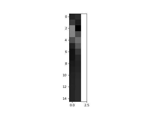
Now, what happens if we replace hrf2, by just the part of hrf2, that cannot be explained by hrf1? Our second regressor is now hrf2 orthogonalized with respect to hrf1:

>>> X_both_o = np.vstack((hrf1, unique_hrf2, np.ones_like(hrf1))).T
>>> plt.imshow(X_both_o, interpolation='nearest', cmap='gray')
<...>

(png, hires.png, pdf)

>>> plt.plot(times, X_both_o[:,0], times, X_both_o[:,1])
[...]

(png, hires.png, pdf)

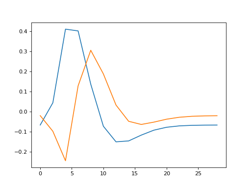
What will happen when we fit this model?

>>> B_boths_o = npl.pinv(X_both_o).dot(Ys)
>>> # Distribution of parameter for hrf1 in orth model
>>> plt.hist(B_boths_o[0], bins=50)
(...)
>>> print(np.mean(B_boths_o[0]), np.std(B_boths_o[0]))
1.68134012906 1.47669405469

(png, hires.png, pdf)

>>> # Predicted variance of hrf1 parameter is the same as for the
>>> # model with hrf1 on its own
>>> np.sqrt(C_both.T.dot(npl.pinv(X_both_o.T.dot(X_both_o)).dot(C_both)))
array([[ 1.485]])

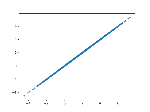
The parameter for the hrf1 regressor has now returned to the same value and variance as it had when hrf1 was the only regressor in the model (apart from the mean). For the orthogonalized model, we removed the part of hrf2 that could be explained by hrf1. Now, the amount of hrf1, that we could find in hrf2, has been added back to the parameter for hrf1, in order to make the fitted \(\hat{y}\) values the same as for the model with both HRFs.

>>> np.mean(B_boths[0, :]) + B_hrf1_in_hrf2
array([ 1.6711])

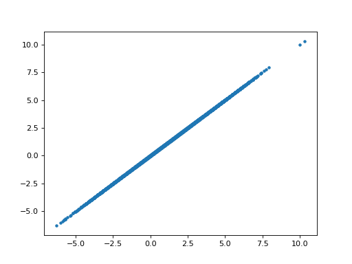
The hrf1 parameter in the orthogonalized model is the same as for the model that only includes hrf1 - as if the orthogonalized hrf2 was not present. The parameter for orthogonalized hrf2 is the same as the parameter for hrf2 in the not-orthogonalized model. We still need the same amount of the orthogonal part of the second regressor to explain the signal:

>>> # Example parameters from the single model
>>> B_ones[:,:5]
array([[ 2.5395, -1.7854,  0.1398,  1.6884,  4.5348],
       [-0.1606, -0.0069,  0.3315, -0.1837, -0.2644]])

>>> # Example parameters from the non-orth model
>>> B_boths[:,:5]
array([[ 2.0143, -2.4845, -2.5391, -0.9706,  4.9768],
       [ 0.7481,  0.9955,  3.815 ,  3.7866, -0.6295],
       [-0.1606, -0.0069,  0.3315, -0.1837, -0.2644]])

>>> # Example parameters from the orth model
>>> B_boths_o[:,:5]
array([[ 2.5395, -1.7854,  0.1398,  1.6884,  4.5348],
       [ 0.7481,  0.9955,  3.815 ,  3.7866, -0.6295],
       [-0.1606, -0.0069,  0.3315, -0.1837, -0.2644]])

>>> # The parameter for the hrf1 regressor in the orth model
>>> # is the same as the parameter for the hrf1 regressor in the
>>> # single regressor model
>>> plt.plot(B_ones[0], B_boths_o[0], '.')
[...]
>>> np.allclose(B_ones[0], B_boths_o[0])
True

(png, hires.png, pdf)

>>> # The parameter for the orthogonalized hrf2 regressor is the same as the
>>> # parameter for the non-orthogonalize hrf2 regressor in the
>>> # non-orthogonalized model
>>> plt.plot(B_boths[1], B_boths_o[1], '.')
[...]
>>> np.allclose(B_boths[1], B_boths_o[1])
True

(png, hires.png, pdf)

>>> # The parameter for the hrf1 regressor in the non-orth model
>>> # is correlated with the parameter for the hrf1 regressor
>>> # in the orth model.
>>> plt.plot(B_boths[0], B_boths_o[0], '.')
[...]
>>> np.corrcoef(B_boths[0], B_boths_o[0])
array([[ 1.    ,  0.7128],
       [ 0.7128,  1.    ]])

(png, hires.png, pdf)

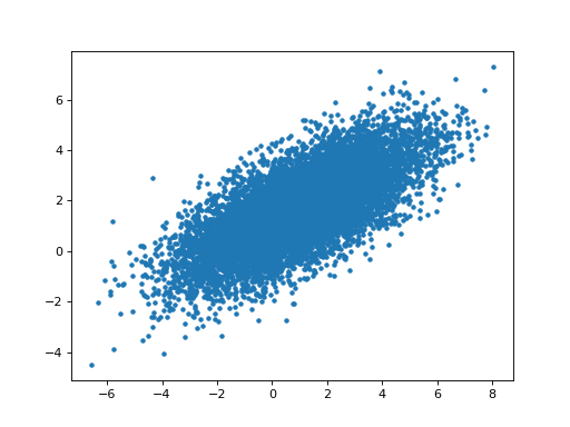
>>> # Relationship of estimated parameters for hrf1 and orthogonalized hrf2
>>> # (they should be independent)
>>> plt.plot(B_boths_o[0], B_boths_o[1], '+')
[...]
>>> np.corrcoef(B_boths_o[0], B_boths_o[1])
array([[ 1.    , -0.0053],
       [-0.0053,  1.    ]])

(png, hires.png, pdf)

• Download this page as a Python code file;

• Download this page as a Jupyter notebook (no outputs).