\(\newcommand{L}[1]{\| #1 \|}\newcommand{VL}[1]{\L{ \vec{#1} }}\newcommand{R}[1]{\operatorname{Re}\,(#1)}\newcommand{I}[1]{\operatorname{Im}\, (#1)}\)

Thresholding with random field theory

You can read this page without knowing any Python programming, by skipping over the code, but reading the code will often help understand the ideas.

I based the page on my understanding of the 1992 paper by Keith Worsley (see refs below). For me, this paper is the most comprehensible paper on random fields in neuroimaging. Please refer to this paper and the Worsley 1996 paper for more detail.

An earlier version of this page became the Random fields introduction chapter in the book Human Brain Function second edition.

The problem

Most statistics packages for functional imaging data create statistical parametric maps. These maps have a value for a certain statistic at each voxel in the brain, which is the result of the statistical test done on the scan data for that voxel, across scans. \(t\) values and \(F\) values are the most common.

For the sake of simplicity, I’ll assume that we have \(Z\) values instead of \(t\) or \(F\) values. \(Z\) values are values from the standard normal distribution. The same sort of arguments apply to \(t\) and \(F\) values, just with slightly different formulae.

The null hypothesis for a particular statistical comparison probably will be that there is no change anywhere in the brain. For example, in a comparison of activation against rest, the null hypothesis would be that there are no differences between the scans in the activation condition, and the scans in the rest condition. This null hypothesis implies that the whole brain volume full of statistic values for the comparison will be similar to a equivalent set of values from a random distribution.

The multiple comparison problem

Given we have a brain full of \(Z\) values, how do we decide whether some of the \(Z\) values are larger (more positive) than we would expect in a similar volume of random numbers? So, in a typical brain volume, we have, say, 200000 voxels and therefore 200000 \(Z\) scores. Because we have so many \(Z\) scores, even if the null hypothesis is true, we can be confident that some of these \(Z\) scores will appear to be significant at standard statistical thresholds for the the individual \(Z\) scores. For example, \(p\) value thresholds such as \(p<0.05 \) or \(p<0.01 \) correspond to \(Z = 1.64 \) and \(Z = 2.33 \) respectively.

>>> import numpy as np
>>> import matplotlib.pyplot as plt
>>> # Tell numpy to print numbers to 4 decimal places only
>>> np.set_printoptions(precision=4, suppress=True)

Hint

If running in the IPython console, consider running %matplotlib to enable interactive plots. If running in the Jupyter Notebook, use %matplotlib inline.

>>> import scipy.stats
>>> normal_distribution = scipy.stats.norm()
>>> # The inverse normal CDF
>>> inv_n_cdf = normal_distribution.ppf
>>> inv_n_cdf([0.95, 0.99])
array([ 1.6449,  2.3263])

So, if we threshold our brain \(Z\) scores at \(2.33 \) or above, we would expect a number of false positives, even if the null hypothesis is true. So, how high should we set our \(Z\) threshold, so that we can be confident that the remaining peak \(Z\) scores are indeed too high to be expected by chance? This is the multiple comparison problem.

We could call all the \(Z\) scores in the brain a “family” of tests. We want to find a threshold so that we can correct for a whole “family” of tests. For this reason, these multiple comparison correction methods are often known as family-wise correction methods.

Why not a Bonferroni correction?

The problem of false positives with multiple statistical tests is an old one. One standard method for dealing with this problem is to use the Bonferroni correction. For the Bonferroni correction, you set your p value threshold for accepting a test as being significant as \(alpha\) / (number of tests), where \(alpha\) is the false positive rate you are prepared to accept. \(alpha\) is often 0.05, or one false positive in 20 repeats of your experiment. Thus, for a statistical map with 200000 voxels, the Bonferroni corrected p value would be 0.05 / 200000 = [equivalent Z] 5.03. We could then threshold our Z map to show us only Z scores higher than 5.03, and be confident that all the remaining Z scores are unlikely to have occurred by chance. For some functional imaging data this is a perfectly reasonable approach, but in most cases the Bonferroni threshold will be considerably too conservative. This is because, for most stastistic maps, the Z scores at each voxel are highly correlated with their neighbours.

Spatial correlation

Functional imaging data usually have some spatial correlation. By this, we mean that data in one voxel are correlated with the data from the neighbouring voxels. This correlation is caused by several factors:

• With low resolution imaging such as PET, data from an individual voxel will contain some signal from the tissue around that voxel;

• Unmodeled brain activation signal, which is very common, will tend to cover several voxels and induce correlations between them;

• Resampling of the images during preprocessing causes some smoothing across voxels;

• Most neuromaging statistical analyses work on smoothed images, and this creates strong spatial correlation. Smoothing is often used to improve signal to noise according to the matched filter theorem (the signal we are looking for is almost invariably spread across several voxels).

The reason this spatial correlation is a problem for the Bonferroni correction is that the Bonferroni correction assumes that you have performed some number of independent tests. If the voxels are spatially correlated, then the \(Z\) scores at each voxel are not independent. This will make the correction too conservative.

Spatial correlation and independent observations

An example can show why the Bonferroni correction is too conservative with non-independent tests. Let us first make an example image out of random numbers. We generate 16384 random numbers, and then put them into a 128 by 128 array. This results in a 2D image of spatially independent random numbers.

>>> # Constants for image simulations etc
>>> shape = [128, 128] # No of pixels in X, Y
>>> n_voxels = np.prod(shape) # Total pixels
>>> s_fwhm = 8 # Smoothing in number of pixels in x, y
>>> seed = 1939 # Seed for random no generator
>>> alpha = 0.05 # Default alpha level
>>>
>>> # Image of independent random nos
>>> np.random.seed(seed) # Seed the generator to get same numbers each time
>>> test_img = np.random.standard_normal(shape)
>>> plt.imshow(test_img)
<...>
>>> plt.set_cmap('bone')
>>> plt.xlabel('Pixel position in X')
<...>
>>> plt.ylabel('Pixel position in Y')
<...>
>>> plt.title('Image 1 - array of independent random numbers')
<...>

(png, hires.png, pdf)

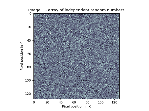
In this picture, whiter pixels are more positive, darker pixels more negative.

The Bonferroni correction is the right one for this image, because the image is made up of 128*128 = 16384 random numbers from a normal distribution. Therefore, from the Bonferroni correction (\(\alpha / N = 0.05 / 16384\) = [Z equivalent] 4.52), we would expect only 5 out of 100 such images to have one or more random numbers in the whole image larger than 4.52.

>>> # Bonferroni threshold for this image
>>> bonf_thresh = inv_n_cdf(1 - (alpha / n_voxels))
>>> print(bonf_thresh)
4.52277137559

The situation changes if we add some spatial correlation to this image. We can take our image above, and perform the following procedure:

• Break up the image into 8 by 8 squares;

• For each square, calculate the mean of all 64 random numbers in the square;

• Replace the 64 random numbers in the square by the mean value.

(In fact, we have one more thing to do to our new image values. When we take the mean of 64 random numbers, the mean and variance will tend to zero. We have therefore to multiply our mean numbers by 8 to restore a variance of 1. This will make the numbers correspond to the normal distribution again. Why 8? Because the variance of the mean of 64 numbers with variance 1 is 1/64, and so we need to multiply the numbers by \(\sqrt{64}\) to restore a variance of 1. See: Sum of uncorrelated variables).

The following is the image that results from the procedure above applied to our first set of random numbers:

>>> # Divide into FWHM chunks and fill square from mean value
>>> sqmean_img = test_img.copy()
>>> for i in range(0, shape[0], s_fwhm):
...     i_slice = slice(i, i+s_fwhm)
...     for j in range(0, shape[1], s_fwhm):
...         j_slice = slice(j, j+s_fwhm)
...         vals = sqmean_img[i_slice, j_slice]
...         sqmean_img[i_slice, j_slice] = vals.mean()
>>> # Multiply up to unit variance again
>>> sqmean_img *= s_fwhm
>>> # Show as image
>>> plt.imshow(sqmean_img)
<...>
>>> plt.set_cmap('bone')
>>> plt.xlabel('Pixel position in X')
<...>
>>> plt.ylabel('Pixel position in Y')
<...>
>>> plt.title('Taking means over %s by %s elements from image 1' % (s_fwhm, s_fwhm))
<...>

(png, hires.png, pdf)

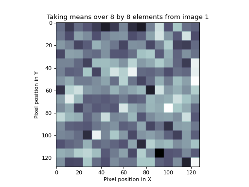
We still have 16384 numbers in our image. However, it is clear that we now have only (128 / 8) * (128 / 8) = 256 independent numbers. The appropriate Bonferroni correction would then be (\(\alpha / N\) = 0.05 / 256 = [\(Z\) equivalent] 3.55). We would expect that if we took 100 such mean-by-square-processed random number images, then only 5 of the 100 would have a square of values greater than 3.55 by chance. However, if we took the original Bonferroni correction for the number of pixels rather than the number of independent pixels, then our \(Z\) threshold would be far too conservative.

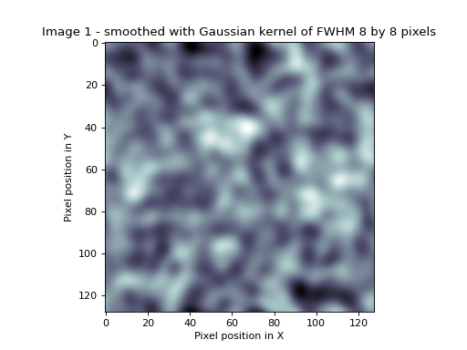
Smoothed images and independent observations

The mean-by-square process we have used above is a form of smoothing. In the mean-by-square case, the averaging takes place only within the squares, but in the case of smoothing with a smoothing kernel, the averaging takes place in a continuous way across the image. We can smooth our first random number image with a Gaussian kernel of FWHM 8 by 8 pixels. (As for the mean-by-square example, the smoothing reduces the variance of the numbers in the image, because an average of random numbers tends to zero. In order to return the variance of the numbers in the image to one, to match the normal distribution, the image must be multiplied by a scale factor. The derivation of this scaling factor is rather technical, and not relevant to the discussion here).

>>> # smooth random number image
>>> import scipy.ndimage as spn
>>> sd = s_fwhm / np.sqrt(8.*np.log(2)) # sigma for this FWHM
>>> stest_img = spn.filters.gaussian_filter(test_img, sd, mode='wrap')
>>>
>>> def gauss_2d_varscale(sigma):
...     """ Variance scaling for smoothing with 2D Gaussian of sigma `sigma`
...
...     The code in this function isn't important for understanding
...     the rest of the tutorial.
...     """
...     # Make a single 2D Gaussian using given sigma
...     limit = sigma * 5 # go to limits where Gaussian will be at or near 0
...     x_inds = np.arange(-limit, limit+1)
...     y_inds = x_inds # Symmetrical Gaussian (sd same in X and Y)
...     [x,y] = np.meshgrid(y_inds, x_inds)
...     # http://en.wikipedia.org/wiki/Gaussian_function#Two-dimensional_Gaussian_function
...     gf    = np.exp(-(x*x + y*y) / (2 * sigma ** 2))
...     gf    = gf/np.sum(gf)
...     # Expectation of variance for this kernel
...     AG    = np.fft.fft2(gf)
...     Pag   = AG * np.conj(AG) # Power of the noise
...     COV   = np.real(np.fft.ifft2(Pag))
...     return COV[0, 0]
...
>>> # Restore smoothed image to unit variance
>>> svar = gauss_2d_varscale(sd)
>>> scf = np.sqrt(1 / svar)
>>> stest_img = stest_img * scf
>>>
>>> # display smoothed image
>>> plt.imshow(stest_img)
<...>
>>> plt.set_cmap('bone')
>>> plt.xlabel('Pixel position in X')
<...>
>>> plt.ylabel('Pixel position in Y')
<...>
>>> plt.title('Image 1 - smoothed with Gaussian kernel of FWHM %s by %s pixels' %
...           (s_fwhm, s_fwhm))
<...>

(png, hires.png, pdf)

In our smoothed image, as for the mean-by-square image, we no longer have 16384 independent observations, but some smaller number, because of the averaging across pixels. If we knew how many independent observations there were, we could use a Bonferroni correction as we did for the mean-by-square example. Unfortunately it is not easy to work out how many independent observations there are in a smoothed image. So, we must take a different approach to determine our \(Z\) score threshold. One approach used by SPM and other packages is to use Random Field Theory (RFT).

Using random field theory

You can think of the application of RFT as proceeding in three steps. First, you determine how many resels there are in your image. Then you use the resel count and some sophisticated maths to work out the expected Euler characteristic (EC) of your image, when it is thresholded at various levels. These expected ECs can be used to give the correct threshold for the required control of false positives (\(\alpha\)).

What is a resel?

A resel is a “resolution element”. The number of resels in an image is similar to the number of independent observations in the image. However, they are not the same, as we will see below. A resel is defined as a block of pixels of the same size as the FWHM of the smoothness of the image. In our smoothed image above, the smoothness of the image is 8 pixels by 8 pixels (the smoothing that we applied). A resel is therefore a 8 by 8 pixel block, and the number of resels in our image is (128 / 8) * (128 / 8) = 256. Note that the number of resels depends only on the number of pixels, and the FWHM.

>>> # No of resels
>>> resels = np.prod(np.array(shape) / float(s_fwhm))
>>> resels
256.0

What is the Euler characteristic?

The Euler characteristic of an image is a property of the image after it has been thresholded. For our purposes, the EC can be thought of as the number of blobs in an image after it has been thresholded. This is best explained by example. Let us take our smoothed image, and threshold it at \(Z > 2.75\). This means we set to zero all the pixels with \(Z\) scores less than or equal to 2.75, and set to one all the pixels with \(Z\) scores greater than 2.75.

We make a function to show the thresholded image:

>>> def show_threshed(img, th):
...     thimg = (img > th)
...     plt.figure()
...     plt.imshow(thimg)
...     plt.set_cmap('bone')
...     plt.xlabel('Pixel position in X')
...     plt.ylabel('Pixel position in Y')
...     plt.title('Smoothed image thresholded at Z > %s' % th)

>>> # threshold at 2.75 and display
>>> show_threshed(stest_img, 2.75)

(png, hires.png, pdf)

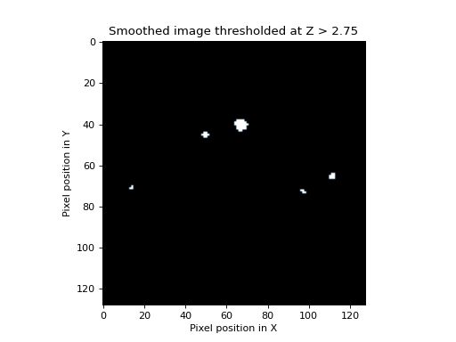
Zero in the image displays as black and one as white. In this picture, there are some blobs, corresponding to areas with \(Z\) scores higher than 2.75. The EC of this image is just the number of blobs. If we increase the threshold to \(3.25\), we find that some of the blobs disappear (the highest \(Z\) values at the blob peaks were less than 3.25).

>>> # threshold at 3.25 and display
>>> show_threshed(stest_img, 3.25)

(png, hires.png, pdf)

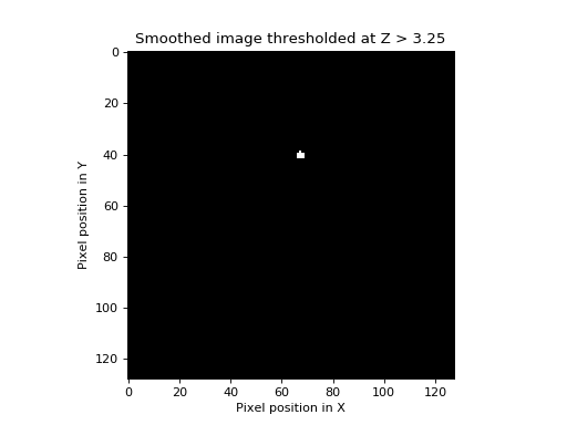
One blob remains; the EC of the image above is therefore 1. It turns out that if we know the number of resels in our image, it is possible to estimate the most likely value of the EC at any given threshold. The formula for this estimate, for two dimensions, is on page 906 of Worsley 1992, implemented below. The graph shows the expected EC of our smoothed image, of 256 resels, when thresholded at different \(Z\) values.

>>> # expected EC at various Z thresholds, for two dimensions
>>> Z = np.linspace(0, 5, 1000)

>>> def expected_ec_2d(z, resel_count):
...     # From Worsley 1992
...     z = np.asarray(z)
...     return (resel_count * (4 * np.log(2)) * ((2*np.pi)**(-3./2)) * z) * np.exp((z ** 2)*(-0.5))
...
>>> expEC = expected_ec_2d(Z, resels)
>>> plt.plot(Z, expEC)
[...]
>>> plt.xlabel('Z score threshold')
<...>
>>> plt.ylabel('Expected EC for thresholded image')
<...>
>>> plt.title('Expected EC for smoothed image with %s resels' % resels)
<...>

(png, hires.png, pdf)

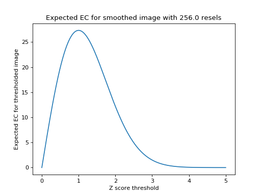
Note that the graph does a reasonable job of predicting the EC in our image; at \(Z = 2.75\) threshold it predicted an EC of 2.8, and at a \(Z = 3.25 \) it predicted an EC of 0.74

>>> expected_ec_2d([2.75, 3.25], resels)
array([ 2.825 ,  0.7449])

How does the Euler characteristic give a Z threshold?

The useful feature of the expected EC is this: when the \(Z\) thresholds become high and the predicted EC drops towards zero, the expected EC is a good approximation of the probability of observing one or more blobs at that threshold. So, in the graph above, when the \(Z\) threshold is set to 4, the expected EC is 0.06. This can be rephrased thus: the probability of getting one or more regions where \(Z\) is greater than 4, in a 2D image with 256 resels, is 0.06. So, we can use this for thresholding. If \(x\) is the \(Z\) score threshold that gives an expected EC of 0.05, then, if we threshold our image at \(x\), we can expect that any blobs that remain have a probability of less than or equal to 0.05 that they have occurred by chance. The threshold \(x\) depends only on the number of resels in our image.

Is the threshold accurate? Show me!

We can test the treshold with a simulation:

>>> # Simulation to test the RFT threshold.
>>> # Find approx threshold from the vector above.
>>> # We're trying to find the Z value for which the expected EC is 0.05
>>> tmp = (Z > 3) & (expEC<=alpha)
>>> alphaTH = Z[tmp][0]
>>> print('Using Z threshold of %f' % alphaTH)
Using Z threshold of 4.054054
>>> # Make lots of smoothed images and find how many have one or more
>>> # blobs above threshold
>>> repeats = 1000
>>> falsepos = np.zeros((repeats,))
>>> maxes = np.zeros((repeats,))
>>> edgepix = s_fwhm  # to add edges to image - see below
>>> big_size = [s + edgepix * 2 for s in shape]
>>> i_slice = slice(edgepix + 1, shape[0] + edgepix + 1)
>>> j_slice = slice(edgepix + 1, shape[1] + edgepix + 1)
>>> for i in range(repeats):
...     # Make random square with extra edges to throw away
...     timg = np.random.standard_normal(size=big_size)
...     stimg = spn.filters.gaussian_filter(timg, sd, mode='wrap')
...     # throw away edges to avoid artefactually high values
...     # at image edges generated by the smoothing
...     stimg = stimg[i_slice, j_slice]
...     # Reset variance using scale factor from calculation above
...     stimg *= scf
...     falsepos[i] = np.any(stimg >= alphaTH)
...     maxes[i] = stimg.max()
>>> print('False positive rate in simulation was %s (%s expected)' %
...       (sum(falsepos) / float(repeats), alpha))
False positive rate in simulation was 0.049 (0.05 expected)

How does the random field correction compare to the Bonferroni correction?

I stated above that the resel count in an image is not exactly the same as the number of independent observations. If it was the same, then instead of using RFT for the expected EC, we could use a Bonferroni correction for the number of resels. However, these two corrections give different answers. Thus, for an alpha of 0.05, the \(Z\) threshold according to RFT, for our 256 resel image, is \(Z=4.05\). However, the Bonferroni threshold, for 256 independent tests, is 0.05/256 = [\(Z\) equivalent] 3.55. So, although the RFT maths gives us a Bonferroni-like correction, it is not the same as a Bonferroni correction. As you can see from the simulation above, the random field correction gives a threshold very close the the observed value for a sequence of smoothed images. A Bonferroni correction with the resel count gives a much lower threshold and would therefore be way off the correct threshold for 0.05 false positive rate.

To three dimensions

Exactly the same principles apply to a smoothed random number image in three dimensions. In this case, the EC is the number of 3D blobs - perhaps “globules” - of \(Z\) scores above a certain threshold. Pixels might better be described as voxels (pixels with volume). The resels are now in 3D, and one resel is a cube of voxels that is of size (FWHM in x) by (FWHM in y) by (FWHM in z). The formula for the expected EC is different in the 3D case, but still depends only on the resels in the image. If we find the threshold giving an expected EC of 0.05, in 3D, we have a threshold above which we can expect that any remaining \(Z\) scores are unlikely to have occurred by chance, with a \(p<0.05\).

More sophisticated random fielding

Random fields and search volumes

I oversimplified when I said above that the expected EC depends only on the number of resels in the image. In fact, this is an approximation, which works well when the volume that we are looking at has a reasonable number of resels. This is true for our two dimensional example, where the FWHM was 8 and our image was 128 by 128. However, the precise EC depends not only on the number of resels, but the shape of the volume in which the resels are contained. It is possible to derive a formula for the expected EC, based on the number of resels in the area we are thresholding, and the shape of the area (see Worsley 1996). This formula is more precise than the formula taking account of the number of resels alone. When the area to be thresholded is large, compared to the FWHM, as is the case when we are thresholding the whole brain, the two formulae give very similar results. However, when the volume for thresholding is small, the formulae give different results, and the shape of the area must be taken into account. This is the case when you require a threshold for a small volume, such as a region of interest.

t and F statistic volumes

Keith Worsley’s 1996 paper gives the random field formulae for \(t\) and \(F\) statistics. SPM and other imaging packages generate \(t\) and \(F\) statistics maps. They use the random fields formulae for \(t\), \(F\) to work out the corrected (family-wise) error rate at each \(t\), \(F\) value.

Estimated instead of assumed smoothness

SPM and other packages also estimate how smooth the images are, rather than assuming the smoothness as we have done here. SPM in particular looks at the the residuals from the statistical analysis to calculate the smoothness of the image, in terms of FWHM. From these calculations it derives estimates for the FWHM in x, y and z. Other than this, the corrected statistics are calculated just as described above.

A brain activation example in SPM

Here is an SPM8 results printout for a first level FMRI analysis.

You will see the FWHM values at the bottom of the page - here they are 4.1 voxels in x, 4.0 voxels in y, and 4.1 voxels in z. These values are rounded; I can get the exact values from MATLAB by looking at xSPM.FWHM. These are:

>>> FWHM = [4.0528, 4.0172, 4.1192]

A resel is therefore a block of volume approx:

>>> resel_volume = np.prod(FWHM)
>>> print(resel_volume)
67.0643168927

That’s the value you see at the bottom the SPM printout after resel =. The resel count of 592.9 in the printout comes from a calculation based on this estimated FWHM smoothness and the shape of the brain. In other words it applies the search volume correction I mentioned above. If it did not apply this correction then the resel count would simply be the number of voxels divided by the resel volume:

>>> print(44532 / resel_volume)
664.019288697

The table gives statistics for each detected cluster in the analysis, ordered by significance level. Each line in bold in the table is the peak voxel for a particular cluster. Lines in standard type are sub-clusters within the same cluster.

Look at the peak voxel for the third-most significant cluster. This is the third bold line in the table, and the seventh line overall. On the left-hand side of the table, you see the values for the “peak-level” statistics. The extreme left gives the voxel location in millimeters. Our voxel of interest is at location x=-42, y=18, z=3.

The value in the “T” column for this voxel is 4.89. This is the raw \(t\) statistic. The column \(P_{FWE-corr}\) gives the random field corrected \(p\) value. In this case the value is 0.037. 0.037 is the expected EC, in a 3D image of 592.9 resels when thresholded at \(t = 4.89\). This is equivalent to saying that the probability of getting one or more blobs of \(t\) value 4.89 or greater, is 0.037.

There are other corrected \(p\) values here, based on cluster size, and based on the false discovery rate, but I didn’t cover those corrections here.

References

Worsley, K.J., Marrett, S., Neelin, P., and Evans, A.C. (1992). A three-dimensional statistical analysis for CBF activation studies in human brain Journal of Cerebral Blood Flow and Metabolism, 12:900-918.

Worsley, K.J., Marrett, S., Neelin, P., Vandal, A.C., Friston, K.J., and Evans, A.C. (1996). A unified statistical approach for determining significant signals in images of cerebral activation Human Brain Mapping, 4:58-73.

• Download this page as a Python code file;

• Download this page as a Jupyter notebook (no outputs);

• Download this page as a Jupyter notebook (with outputs).