\(\newcommand{L}[1]{\| #1 \|}\newcommand{VL}[1]{\L{ \vec{#1} }}\newcommand{R}[1]{\operatorname{Re}\,(#1)}\newcommand{I}[1]{\operatorname{Im}\, (#1)}\)

Introducing principal component analysis

This page was much inspired by these two excellent tutorials:

• Kendrick Kay’s tutorial on principal component analysis;

• Lior Pachter’s tutorial.

Background

Check that you understand:

• Vector projection;

• matrix multiplication. See this Khan academy introduction to matrix multiplication. I highly recommend Gilbert Strang’s lecture on matrix multiplication.

Setting the scene

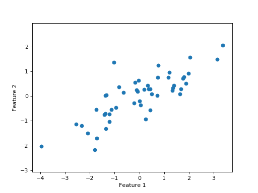
Let’s say I have some data in a 2D array \(\mathbf{X}\).

I have taken two different measures for each sample, and 50 samples. We can also call the measures variables or features. So, I have two features and 50 samples.

I arrange the data so each column is one sample (I have 50 columns). Each row is one feature (or measure or variable) (I have two rows).

Start by loading the libraries we need, and doing some configuration:

>>> import numpy as np
>>> import numpy.linalg as npl
>>> # Display array values to 6 digits of precision
>>> np.set_printoptions(precision=6, suppress=True)

Hint

If running in the IPython console, consider running %matplotlib to enable interactive plots. If running in the Jupyter Notebook, use %matplotlib inline.

Make the data:

>>> # Make some random, but predictable data
>>> np.random.seed(1966)
>>> X = np.random.multivariate_normal([0, 0], [[3, 1.5], [1.5, 1]], size=50).T
>>> X.shape
(2, 50)

To make things simpler, I will subtract the mean across samples from each feature. As each feature is one row, I need to subtract the mean of each row, from each value in the row:

>>> # Subtract mean across samples (mean of each feature)
>>> x_mean = X.mean(axis=1)
>>> X[0] = X[0] - x_mean[0]
>>> X[1] = X[1] - x_mean[1]

The values for the two features (rows) in \(\mathbf{X}\) are somewhat correlated:

(png, hires.png, pdf)

We want to explain the variation in these data.

The variation we want to explain is given by the sum of squares of the data values.

>>> squares = X ** 2
>>> print(np.sum(squares))
155.669289858

The sums of squares of the data can be thought of as the squared lengths of the 50 2D vectors in the columns of \(\mathbf{X}\).

We can think of each sample as being a point on a 2D coordinate system, where the first feature is the position on the x axis, and the second is the position on the y axis. In fact, this is how we just plotted the values in the scatter plot. We can also think of each column as a 2D vector. Call \(\vec{v_j}\) the vector contained in column \(j\) of matrix \(\mathbf{X}\), where \(j \in 1..50\).

The sum of squares across the features, is also the squared distance of the point (column) from the origin (0, 0). That is the same as saying that the sum of squares is the squared length of \(\vec{v_j}\). This can be written as \(\|\vec{v_j}\|^2\)

Take the first column / point / vector as an example (\(\vec{v_1}\)):

>>> v1 = X[:, 0]
>>> v1
array([ 3.378322,  2.068158])

(png, hires.png, pdf)

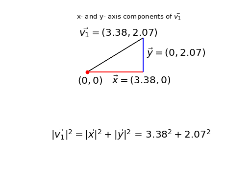
So, the sums of squares we are trying to explain can be expressed as the sum of the squared distance of each point from the origin, where the points (vectors) are the columns of \(\mathbf{X}\):

(png, hires.png, pdf)

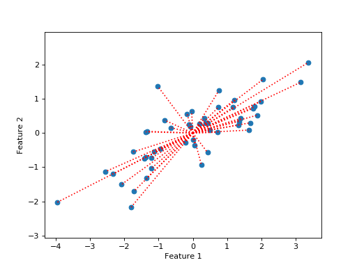
Put another way, we are trying to explain the squares of the lengths of the dotted red lines on the plot.

At the moment, we have not explained anything, so our current unexplained sum of squares is:

>>> print(np.sum(X ** 2))
155.669289858

For the following you will need to know how to use vector dot products to project one vector on another.

See Vectors and dot products and Vector projection for the details, and please try the excellent Khan academy videos linked from those pages if you are new to vector dot products or are feeling rusty.

Let us now say that we want to try and find a line that will explain the maximum sum of squares in the data.

We define our line with a unit vector \(\hat{u}\). All points on the line can be expressed with \(c\hat{u}\) where \(c\) is a scalar.

Our best fitting line \(c\hat{u}\) is the line that comes closest to the points, in the sense of minimizing the squared distance between the line and points.

Put a little more formally, for each point \(\vec{v_j}\) we will find the distance \(d_j\) between \(\vec{v_j}\) and the line. We want the line with the smallest \(\sum_j{d_j^2}\).

What do we mean by the distance in this case? The distance \(d_i\) is the distance between the point \(\vec{v_i}\) and the projection of that point onto the line \(c\hat{u}\). The projection of \(\vec{v_i}\) onto the line defined by \(\hat{u}\) is, as we remember, given by \(c\hat{u}\) where \(c = \vec{v_i}\cdot\hat{u}\).

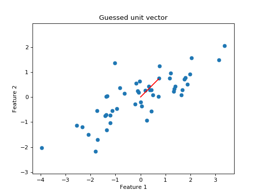
Looking at the scatter plot, we might consider trying a unit vector at 45 degrees angle to the x axis:

>>> u_guessed = np.array([np.cos(np.pi / 4), np.sin(np.pi / 4)])
>>> u_guessed
array([ 0.707107,  0.707107])

This is a unit vector:

>>> np.sum(u_guessed ** 2)
1.0

(png, hires.png, pdf)

Let’s project all the points onto that line:

>>> u_guessed_row = u_guessed.reshape((1, 2))  # A row vector
>>> c_values = u_guessed_row.dot(X)  # c values for scaling u
>>> # scale u by values to get projection
>>> projected = u_guessed_row.T.dot(c_values)

(png, hires.png, pdf)

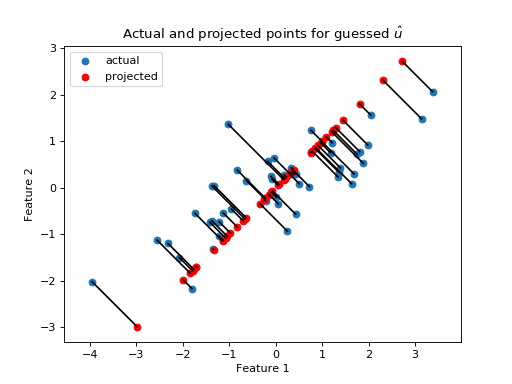
The projected points (in red), are the positions of the points that can be explained by projection onto the guessed line defined by \(\hat{u}\). The red projected points also have their own sum of squares:

>>> print(np.sum(projected ** 2))
133.381320743

Because we are projecting onto a unit vector, \(\|c\hat{u}\|^2 = c\hat{u} \cdot c\hat{u} = c^2(\hat{u} \cdot \hat{u}) = c^2\). Therefore the c_values are also the lengths of the projected vectors, so the sum of squares of the c_values also gives us the sum of squares of the projected points:

>>> print(np.sum(c_values ** 2))
133.381320743

As we will see later, this is the sum of squares from the original points that have been explained by projection onto \(\hat{u}\).

Once I have the projected points, I can calculate the remaining distance of the actual points from the projected points:

>>> remaining = X - projected
>>> distances = np.sqrt(np.sum(remaining ** 2, axis=0))
>>> distances
array([ 0.926426,  0.714267,  0.293125,  0.415278,  0.062126,  0.793188,
        0.684554,  1.686549,  0.340629,  0.006746,  0.301138,  0.405397,
        0.995828,  0.171356,  1.094742,  0.780583,  0.183566,  0.974734,
        0.732008,  0.495833,  0.96324 ,  1.362817,  0.262868,  0.092597,
        0.477803,  0.041519,  0.84133 ,  0.33801 ,  0.019824,  0.853356,
        0.069814,  0.244263,  0.347968,  0.470062,  0.705145,  1.173709,
        0.838709,  1.006069,  0.731594,  0.74943 ,  0.343281,  0.55684 ,
        0.287912,  0.479475,  0.977735,  0.064308,  0.127375,  0.157425,
        0.01017 ,  0.519997])

I can also express the overall (squared) remaining distance as the sum of squares. The following is the code version of the formula \(\sum_j{d_j^2}\) that you saw above:

>>> print(np.sum(remaining ** 2))
22.2879691152

I’m going to try a whole lot of different values for \(\hat{u}\), so I will make a function to calculate the result of projecting the data onto a line defined by a unit vector \(\hat{u}\):

>>> def line_projection(u, X):
...     """ Return columns of X projected onto line defined by u
...     """
...     u = u.reshape(1, 2)  # A row vector
...     c_values = u.dot(X)  # c values for scaling u
...     projected = u.T.dot(c_values)
...     return projected

Next a small function to return the vectors remaining after removing the projections:

>>> def line_remaining(u, X):
...     """ Return vectors remaining after removing cols of X projected onto u
...     """
...     projected = line_projection(u, X)
...     remaining = X - projected
...     return remaining

Using these little functions, I get the same answer as before:

>>> print(np.sum(line_remaining(u_guessed, X) ** 2))
22.2879691152

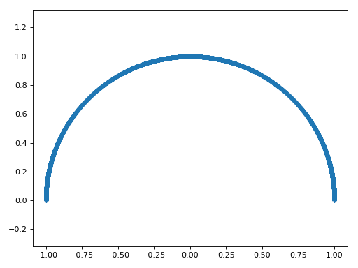
Now I will make lots of \(\hat{u}\) vectors spanning half the circle:

>>> angles = np.linspace(0, np.pi, 10000)
>>> x = np.cos(angles)
>>> y = np.sin(angles)
>>> u_vectors = np.vstack((x, y))
>>> u_vectors.shape
(2, 10000)

>>> plt.plot(u_vectors[0], u_vectors[1], '+')
[...]
>>> plt.axis('equal')
(...)
>>> plt.tight_layout()

(png, hires.png, pdf)

I then get the remaining sum of squares after projecting onto each of these unit vectors:

>>> remaining_ss = []
>>> for u in u_vectors.T: # iterate over columns
...     remaining = line_remaining(u, X)
...     remaining_ss.append(np.sum(remaining ** 2))
>>> plt.plot(angles, remaining_ss)
[...]
>>> plt.xlabel('Angle of unit vector')
<...>
>>> plt.ylabel('Remaining sum of squares')
<...>

(png, hires.png, pdf)

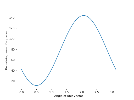
It looks like the minimum value is for a unit vector at around angle 0.5 radians:

>>> min_i = np.argmin(remaining_ss)
>>> angle_best = angles[min_i]
>>> print(angle_best)
0.498620616186

>>> u_best = u_vectors[:, min_i]
>>> u_best
array([ 0.878243,  0.478215])

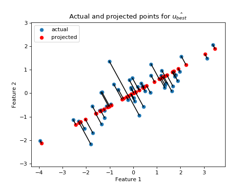
I plot the data with the new unit vector I found:

(png, hires.png, pdf)

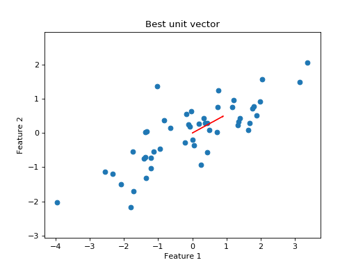
Do the projections for this best line look better than before?

>>> projected = line_projection(u_best, X)

(png, hires.png, pdf)

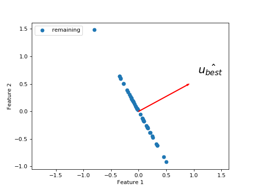
Now we have found a reasonable choice for our first best fitting line, we have a set of remaining vectors that we have not explained. These are the vectors between the projected and actual points.

>>> remaining = X - projected

(png, hires.png, pdf)

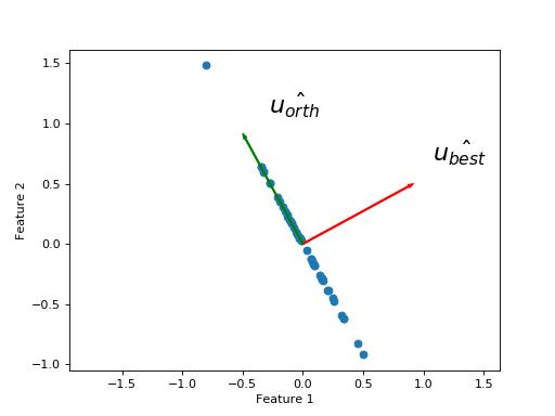
What is the next line we need to best explain the remaining sum of squares? We want another unit vector orthogonal to the first. This is because we have already explained everything that can be explained along the direction of \(\hat{u_{best}}\), and we only have two dimensions, so there is only one remaining direction along which the variation can occur.

I get the new \(\hat{u_{orth}}\) vector with a rotation by 90 degrees (\(\pi / 2\)):

>>> u_best_orth = np.array([np.cos(angle_best + np.pi / 2), np.sin(angle_best + np.pi / 2)])

Within error due to the floating point calculations, \(\hat{u_{orth}}\) is orthogonal to \(\hat{u_{best}}\):

>>> np.allclose(u_best.dot(u_best_orth), 0, atol=1e-6)
True

(png, hires.png, pdf)

The projections onto \(\hat{u_{orth}}\) are the same as the remaining points, because the remaining points already lie along the line defined by \(\hat{u_{orth}}\).

>>> projected_onto_orth = line_projection(u_best_orth, remaining)
>>> np.allclose(projected_onto_orth, remaining)
True

If we have really found the line \(\hat{u_{best}}\) that removes the most sum of squares from the remaining points, then this is the first principal component of \(\mathbf{X}\). \(\hat{u_{orth}}\) will be the second principal component of \(\mathbf{X}\).

Now for a trick. Remember that the two principal components are orthogonal to one another. That means, that if I project the data onto the second principal component \(\hat{u_{orth}}\), I will (by the definition of orthogonal) pick up no component of the columns of \(\mathbf{X}\) that is colinear (predictable via projection) with \(\hat{u_{best}}\).

This means that I can go straight to the projection onto the second component, from the original array \(\mathbf{X}\).

>>> # project onto second component direct from data
>>> projected_onto_orth_again = line_projection(u_best_orth, X)
>>> # Gives same answer as projecting remainder from first component
>>> np.allclose(projected_onto_orth_again, projected_onto_orth)
True

\(\newcommand{\X}{\mathbf{X}}\newcommand{\U}{\mathbf{U}}\newcommand{\S}{\mathbf{\Sigma}}\newcommand{\V}{\mathbf{V}}\newcommand{\C}{\mathbf{C}}\) For the same reason, I can calculate the scalar projections \(c\) for both components at the same time, by doing matrix multiplication. First assemble the components into the columns of a 2 by 2 array \(\U\):

>>> # Components as columns in a 2 by 2 array
>>> U = np.column_stack((u_best, u_best_orth))
>>> U
array([[ 0.878243, -0.478215],
       [ 0.478215,  0.878243]])

Call the 2 by 50 scalar projection values matrix \(\C\). I can calculate \(\C\) in one shot by matrix multiplication:

\[\C = \U^T \X\]

>>> C = U.T.dot(X)

The first row of \(\C\) has the scalar projections for the first component (the first component is the first column of \(\U\)). The second row has the scalar projections for the second component.

Finally, we can get the projections of the vectors in \(\X\) onto the components in \(\U\) by taking the dot products of the columns in \(\U\) with the scalar projections in \(\C\):

>>> # Result of projecting on first component, via array dot
>>> # np.outer does the equivalent of a matrix multiply of a column vector
>>> # with a row vector, to give a matrix.
>>> projected_onto_1 = np.outer(U[:, 0], C[0, :])
>>> # The same as doing the original calculation
>>> np.allclose(projected_onto_1, line_projection(u_best, X))
True

>>> # Result of projecting on second component, via np.outer
>>> projected_onto_2 = np.outer(U[:, 1], C[1, :])
>>> # The same as doing the original calculation
>>> np.allclose(projected_onto_2, line_projection(u_best_orth, X))
True

The principal component lines are new axes to express the data

My original points were expressed in the orthogonal, standard x and y axes. My principal components give new orthogonal axes. When I project, I have just re-expressed my original points on these new orthogonal axes. Let’s call the projections of \(\vec{v_1}\) onto the first and second components: \(proj_1\vec{v_1}\), \(proj_2\vec{v_1}\).

For example, here is my original first point \(\vec{v_1}\) expressed using the projections onto the principal component axes:

(png, hires.png, pdf)

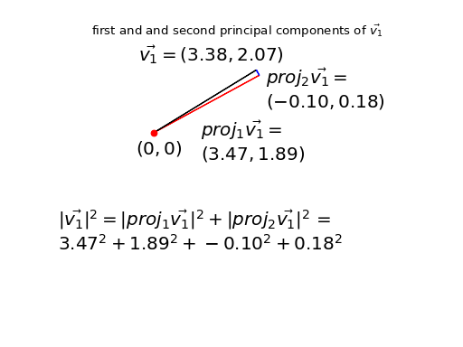
We have re-expressed \(\vec{v_1}\) by two new orthogonal vectors \(proj_1\vec{v_1}\) plus \(proj_2\vec{v_1}\). In symbols: \(\vec{v_1} = proj_1\vec{v_1} + proj_2\vec{v_1}\).

The sum of component 1 projections and the component 2 projections add up to the original vectors (points).

Sure enough, if I sum up the data projected onto the first component and the data projected onto the second, I get back the original data:

>>> np.allclose(projected_onto_1 + projected_onto_2, X)
True

Doing the sum above is the same operation as matrix multiplication of the components \(\U\) with the scalar projections \(\C\). Seeing that this is so involves writing out a few cells of the matrix multiplication in symbols and staring at it for a while.

>>> data_again = U.dot(C)
>>> np.allclose(data_again, X)
True

The components partition the sums of squares

Notice also that I have partitioned the sums of squares of the data into a part that can be explained by the first component, and a part that can be explained by the second:

>>> # Total sum of squares
>>> print(np.sum(X ** 2))
155.669289858

>>> # Sum of squares in the projection onto the first
>>> ss_in_first = np.sum(projected_onto_1 ** 2)
>>> # Sum of squares in the projection onto the second
>>> ss_in_second = np.sum(projected_onto_2 ** 2)
>>> # They add up to the total sum of squares
>>> print((ss_in_first, ss_in_second, ss_in_first + ss_in_second))
(143.97317154347922, 11.696118314873956, 155.66928985835318)

Why is this?

Consider the first vector in \(\mathbf{X}\) : \(\vec{v_1}\). We have re-expressed the squared length of \(\vec{v_1}\) with the squared length of \(proj_1\vec{v_1}\) plus the squared length of \(proj_2\vec{v_1}\). The length of \(\vec{v_1}\) is unchanged, but we now have two new orthogonal vectors making up the sides of the right angled triangle of which \(\vec{v_1}\) is the hypotenuse. The total sum of squares in the data is given by:

\[\begin{split}\sum_j x^2 + \sum_j y^2 = \\ \sum_j \left( x^2 + y^2 \right) = \\ \sum_j \|\vec{v_1}\|^2 = \\ \sum_j \left( \|proj_1\vec{v_1}\|^2 + \|proj_2\vec{v_1}\|^2 \right) = \\ \sum_j \|proj_1\vec{v_1}\|^2 + \sum_j \|proj_2\vec{v_1}\|^2 \\\end{split}\]

where \(j\) indexes samples - \(j \in 1..50\) in our case.

The first line shows the partition of the sum of squares into standard x and y coordinates, and the last line shows the partition into the first and second principal components.

Finding the principal components with SVD

You now know what a principal component analysis is.

It turns out there is a much quicker way to find the components than the slow and dumb search that I did above.

For reasons that we don’t have space to go into, we can get the components using Singular Value Decomposition (SVD) of \(\mathbf{X}\).

See http://arxiv.org/abs/1404.1100 for more detail.

The SVD on an array containing only real (not complex) values such as \(\mathbf{X}\) is defined as:

\[\X = \U \Sigma \V^T\]

If \(\X\) is shape \(M\) by \(N\) then \(\U\) is an \(M\) by \(M\) orthogonal matrix, \(\S\) is a diagonal matrix shape \(M\) by \(N\), and \(\V^T\) is an \(N\) by \(N\) orthogonal matrix.

>>> U, S, VT = npl.svd(X)
>>> U.shape
(2, 2)
>>> VT.shape
(50, 50)

The components are in the columns of the returned matrix \(\U\).

>>> U
array([[-0.878298, -0.478114],
       [-0.478114,  0.878298]])

Remember that a vector \(\vec{r}\) defines the same line as the vector \(-\vec{r}\), so we do not care about a flip in the sign of the principal components:

>>> u_best
array([ 0.878243,  0.478215])

>>> u_best_orth
array([-0.478215,  0.878243])

The returned vector S gives the \(M\) singular values that form the main diagonal of the \(M\) by \(N\) diagonal matrix \(\S\). The values in S give the square root of the explained sum of squares for each component:

>>> S ** 2
array([ 143.973173,   11.696117])

The formula above is for the “full” SVD. When the number of rows in \(\X\) (\(= M\)) is less than the number of columns (\(= N\)) the SVD formula above requires an \(M\) by \(N\) matrix \(\S\) padded on the right with \(N - M\) all zero columns, and an \(N\) by \(N\) matrix \(\V^T\), where the last \(N - M\) rows will be discarded by matrix multiplication with the all zero rows in \(\S\). A variant of the full SVD is the thin SVD, where we discard the useless columns and rows and return \(\S\) as a diagonal matrix \(M x M\) and \(\V^T\) with shape \(M x N\). This is the full_matrices=False variant in NumPy:

>>> U, S, VT = npl.svd(X, full_matrices=False)
>>> U.shape
(2, 2)
>>> VT.shape
(2, 50)

By the definition of the SVD, \(\U\) and \(\V^T\) are orthogonal matrices, so \(\U^T\) is the inverse of \(\U\) and \(\U^T \U = I\). Therefore:

\[\X = \U \Sigma \V^T \implies \U^T \X = \Sigma \V^T\]

You may recognize \(\U^T \X\) as the matrix of scalar projections \(\C\) above:

>>> C = U.T.dot(X)
>>> np.allclose(np.diag(S).dot(VT), C)
True

Because \(\V^T\) is also an orthogonal matrix, it has row lengths of 1, and we can get the values in \(\S\) from the row lengths of \(\C\):

>>> S_from_C = np.sqrt(np.sum(C ** 2, axis=1))
>>> np.allclose(S_from_C, S)
True

Now we can reconstruct \(\V^T\):

>>> # Divide out reconstructed S values
>>> S_as_column = S_from_C.reshape((2, 1))
>>> np.allclose(C / S_as_column, VT)
True

The SVD is quick to compute for a small matrix like X, but when the larger dimension of \(\X\) becomes large, it is more efficient in CPU time and memory to calculate \(\U\) and \(\S\) by doing the SVD on the variance / covariance matrix of the features.

Here’s why that works:

\[\begin{split}\U \S \V^T = \X \\ (\U \S \V^T)(\U \S \V^T)^T = \X \X^T\end{split}\]

By the matrix transpose rule and associativity of matrix multiplication:

\[\U \S \V^T \V \S^T \U^T = \X \X^T\]

\(\V^T\) is an orthogonal matrix, so \(\V^T = \V^{-1}\) and \(\V^T \V = I\). \(\S\) is a diagonal matrix so \(\S \S^T = \S^2\), where \(\S^2\) is a square diagonal matrix shape \(M\) by \(M\) containing the squares of the singular values from \(\S\):

\[\U \S^2 \U^T = \X \X^T\]

This last formula is the formula for the SVD of \(\X \X^T\). So, we can get our \(\U\) and \(\S\) from the SVD on \(\X \X^T\).

>>> # Finding principal components using SVD on X X^T
>>> unscaled_cov = X.dot(X.T)
>>> U_vcov, S_vcov, VT_vcov = npl.svd(unscaled_cov)
>>> U_vcov
array([[-0.878298, -0.478114],
       [-0.478114,  0.878298]])

We know from the derivation above that VT_vcov is just the transpose of \(\U\):

>>> np.allclose(U, VT_vcov.T)
True

The returned vector S_vcov from the SVD on \(\X \X^T\) now contains the explained sum of squares for each component:

>>> S_vcov
array([ 143.973173,   11.696117])

Sums of squares and variance from PCA

We have done the SVD on the unscaled variance / covariance matrix. Unscaled means that the values in the matrix have not been divided by \(N\), or \(N-1\), where \(N\) is the number of samples. This matters little for our case, but sometimes it is useful to think in terms of the variance explained by the components, rather than the sums of squares.

The standard variance of a vector \(\vec{x}\) with \(N\) elements \(x_1, x_2, ... x_N\) indexed by \(i\) is given by \(\frac{1}{N-1} \sum_i \left( x_i - \bar{x} \right)^2\). \(\bar{x}\) is the mean of \(\vec{x}\): \(\bar{x} = \frac{1}{N} \sum_i x_i\). If \(\vec{q}\) already has zero mean, then the variance of \(\vec{q}\) is also given by \(\frac{1}{N-1} \vec{q} \cdot \vec{q}\).

The \(N-1\) divisor for the variance comes from Bessel’s correction for bias.

The covariance between two vectors \(\vec{x}, \vec{y}\) is \(\frac{1}{N-1} \sum_i \left( x_i - \bar{x} \right) \left( y_i - \bar{y} \right)\). If vectors \(\vec{q}, \vec{p}\) already both have zero mean, then the covariance is given by \(\frac{1}{N-1} \vec{q} \cdot \vec{p}\).

Our unscaled variance covariance has removed the mean and done the dot products above, but it has not applied the \(\frac{1}{N-1}\) scaling, to get the true variance / covariance.

For example, the standard numpy covariance function np.cov completes the calculation of true covariance by dividing by \(N-1\).

>>> # Calculate unscaled variance covariance again
>>> unscaled_cov = X.dot(X.T)
>>> # When divided by N-1, same as result of 'np.cov'
>>> N = X.shape[1]
>>> np.allclose(unscaled_cov / (N - 1), np.cov(X))
True

We could have run our SVD on the true variance covariance matrix. The result would give us exactly the same components. This might make sense from the fact that the lengths of the components are always scaled to 1 (unit vectors):

>>> scaled_U, scaled_S, scaled_VT = npl.svd(np.cov(X))
>>> np.allclose(scaled_U, U), np.allclose(scaled_VT, VT_vcov)
(True, True)

The difference is only in the singular values in the vector S:

>>> S_vcov
array([ 143.973173,   11.696117])

>>> scaled_S
array([ 2.938228,  0.238696])

As you remember, the singular values from the unscaled covariance matrix were the sum of squares explained by each component. The singular values from the true covariance matrix are the variances explained by each component. The variances are just the sum of squares divided by the correction in the denominator, in our case, \(N-1\):

>>> S_vcov / (N - 1)
array([ 2.938228,  0.238696])

So far we have described the PCA as breaking up the sum of squares into parts explained by the components. If we do the SVD on the true covariance matrix, then we can describe the PCA as breaking up the variance of the data (across samples) into parts explained by the components. The only difference between these two is the scaling of the S vector.

• Download this page as a Python code file;

• Download this page as a Jupyter notebook (no outputs).