\(\newcommand{L}[1]{\| #1 \|}\newcommand{VL}[1]{\L{ \vec{#1} }}\newcommand{R}[1]{\operatorname{Re}\,(#1)}\newcommand{I}[1]{\operatorname{Im}\, (#1)}\)
The argument in “Why most published research findings are false”
I spent some time trying to understand the argument in this paper:
Ioannidis, John PA. 2005. “Why most published research findings are false.” PLoS medicine 2 (8): e124.
These papers were useful for understanding the argument:
Goodman, Steven, and Sander Greenland. 2007. “Assessing the unreliability of the medical literature: a response to ‘why most published research findings are false.’” Johns Hopkins University, Dept. of Biostatistics Working Papers.
Kass, Robert E., and Adrian E. Raftery. 1995. “Bayes factors.” Journal of the American Statistical Association 90 (430): 773–795.
Wacholder, Sholom, Stephen Chanock, Montserrat Garcia-Closas, Nathaniel Rothman, and others. 2004. “Assessing the probability that a positive report is false: an approach for molecular epidemiology studies.” Journal of the National Cancer Institute 96 (6): 434–442.
“The practice of science is profoundly broken”. Discuss? - no - model and test!
The point that Ioannidis makes is:
We know that the scientific process is flawed in a variety of ways. We assume that these flaws do not have a large effect on the outcome. But, if we model some of the flaws, we see that their effect can be catastrophic, in the sense that a large proportion of scientific findings are likely to be wrong.
We scientists commit ourselves to rational thinking. In this case, rational thinking is asking, “how likely is it that we are getting the answers wrong”?. We have to ask this question in a rational way. This is what Ioannidis sets out to do in this paper.
Different ways of phrasing the argument
The basis of Ioannidis’ argument comes from Wacholder et al 2004 (see appendix table 1). Goodman and Greenland 2007 explain Ioannidis in terms of Bayes theorem.
Both Ioannidis and Goodman & Greenland use odds ratios rather than probability values in their exposition. I found it easier to think in terms of probabilities.
Some terms
We’ve done an experiment, and we have conducted a statistical test:
\(H_A\) - alternative hypothesis
\(H_0\) - null hypothesis
\(\alpha\) : false positive rate - probability for test to reject \(H_0\) when \(H_0\) is true (\(H_A\) is false)
\(\beta\) : false negative rate - probability for test to accept \(H_0\) when \(H_A\) is true (\(H_0\) is false)
\(1 - \beta\) : power - probability we will reject \(H_0\) if \(H_A\) is true (\(H_0\) is false)
Let’s say that the test can either be “significant” (test gives \(p \le \alpha\)) or “not significant” (\(p > \alpha\)). Denote “test is significant” by \(T_S\), “test not significant” by \(T_N\).
Before we did the experiment there were two possibilities - \(H_A\) is true, or \(H_0\) is true. After we have four possibilities:
\(H_A \land T_S\) : \(H_A\) is true, test is significant;
\(H_A \land T_N\) : \(H_A\) is true, test is not significant;
\(H_0 \land T_S\) : \(H_0\) is true (\(H_A\) is false) - test is significant;
\(H_0 \land T_N\) : \(H_0\) is true (\(H_A\) is false) - test is not significant.
What does a “significant” statistical test result tell us?
In this section we work up slowly to Ioannidis table 1.
First we need to load functions for symbolic mathematics from the Sympy library:
>>> from sympy import symbols, Eq, solve, simplify, lambdify, init_printing, latex
>>> init_printing(use_latex=True, order='old')
If we do not take any prior probabilities into account, then we have the following probabilities:
\(\mathtt{\text{T\_S}}\) |
\(\mathtt{\text{T\_N}}\) |
|
\(H_A\) |
\(1 - \beta\) |
\(\beta\) |
\(H_0\) |
\(\alpha\) |
\(1 - \alpha\) |
Total |
\(1 + \alpha - \beta\) |
\(1 + \beta - \alpha\) |
\(\newcommand{Frac}[2]{\frac{\displaystyle #1}{\displaystyle #2}}\)
Some new terms:
\(Pr(H_A)\) - prior probability of \(H_A\) - probability of \(H_A\) before the experiment was conducted.
\(Pr(H_0)\) - prior probability of \(H_0\) = \(1 - Pr(H_A)\) - probability of null hypothesis before experiment conducted
We are interested in updating the probability of \(H_A\) and \(H_0\) as a result of a test on some collected data. This updated probability is \(Pr(H_A | T)\) - the probability of \(H_A\) given the test result \(T\). \(Pr(H_A | T)\) is called the posterior probability because it is the probability after the test result.
The test result \(T\) is assumed to have arisen under either \(H_A\) or \(H_0\).
\(Pr(T) = Pr(T | H_A) Pr(H_A) + Pr(T | H_0) Pr(H_0)\)
Also the probability of a signficant result of the test \(T_S\) is from the same formula:
\(Pr(T_S) = Pr(T_S | H_A) Pr(H_A) + Pr(T_S | H_0) Pr(H_0)\)
(From Kass & Rafferty 1995)
Remembering Bayes theorem:
\(P(A | B) = \Frac{P(B | A) P(A)}{P(B)}\)
Bayes theorem gives:
\(P(H_A | T) = \Frac{Pr(T | H_A) Pr(H_A)}{Pr(T)} = \Frac{Pr(T | H_A) Pr(H_A)}{Pr(T | H_A) Pr(H_A) + Pr(T | H_0) Pr(H_0)}\)
Consider only the test result \(T_S\) (the test is significant). What is the posterior probability of \(H_A\) given that the test is significant?
\(P(H_A | T_S) = \Frac{Pr(T_S | H_A) Pr(H_A)}{Pr(T_S | H_A) Pr(H_A) + Pr(T_S | H_0) Pr(H_0)}\)
We have \(Pr(T_S | H_A)\), \(Pr(T_S | H_0)\) from the first column of the table above. Substituting into the equation:
\(P(H_A | T_S) = \Frac{(1 - \beta) Pr(H_A)}{(1 - \beta) Pr(H_A) + \alpha Pr(H_0)}\)
To make this a little less cluttered, define:
\(\pi := Pr(H_A)\)
So
\(1 - \pi = Pr(H_0)\)
and:
\(P(H_A | T_S) = \Frac{(1 - \beta) \pi}{(1 - \beta) \pi + \alpha (1 - \pi)}\)
Let’s put that formula into Sympy for later:
>>> from sympy.abc import alpha, beta, pi # get symbolic variables
>>> post_prob = (1 - beta) * pi / ((1 - beta) * pi + alpha * (1 - pi))
>>> post_prob
pi*(-beta + 1)/(alpha*(-pi + 1) + pi*(-beta + 1))
A table shows the new probabilities that take the prior into account:
\(\mathtt{\text{T\_S}}\) |
\(\mathtt{\text{T\_N}}\) |
|
\(H_A\) |
\(\pi \left(1 - \beta\right)\) |
\(\beta \pi\) |
\(H_0\) |
\(\alpha \left(1 - \pi\right)\) |
\(\left(1 - \alpha\right) \left(1 - \pi\right)\) |
Total |
\(\alpha \left(1 - \pi\right) + \pi \left(1 - \beta\right)\) |
\(\beta \pi + \left(1 - \alpha\right) \left(1 - \pi\right)\) |
This table is equivalent to Ioannidis table 1. The first column of the table gives the probabilities in the case we’re interested in, of \(T_S\). The posterior probability is the first row, first column - \(Pr(T_S | H_A)\), divided by the total row, first column - \(Pr(T_S)\).
Ioannidis uses “positive predictive value” (PPV) for the posterior probability \(P(H_A | T_S)\). Goodman and Greenland complain, reasonably enough, that “positive predictive value” is a confusing new term for a standard concept.
Ioannidis also prefers his equations in terms of \(R\) - the prior odds ratio. \(R := \Frac{Pr(H_A)}{Pr(H_0)}\). Also (from \(\pi := Pr(H_A)\) and \(Pr(H_0) = 1 - Pr(H_A)\)): \(R = \Frac{\pi}{1 - \pi}\).
Ioannidis’ formula for PPV is \(\Frac{(1 - \beta) R}{R - \beta R + \alpha}\). This is the same as our formula above, only rephrased in terms of \(R\):
>>> R = pi / (1 - pi)
>>> ppv = (1 - beta) * R / (R - beta * R + alpha)
>>> # Is this the same as our formula above?
>>> simplify(ppv - post_prob) == 0
True
The posterior probability is our estimate of whether \(H_A\) is true, given our prior knowledge \(Pr(H_A) = \pi\) combined with the new information from the test result.
What is a finding that is likely to be true?
A finding that is likely to be true is one for which the posterior probability \(Pr(H_A | T_S) > 0.5\). That is, the likelihood of the tested hypothesis, given the reported significant test result, is greater than \(0.5\)
Whether a finding is likely to be true depends on the power of the experiment
Assume that \(\alpha = 0.05\) (standard significance threshold for null hypothesis test).
Let’s have a look at the posterior probability as a function of power and prior probability:
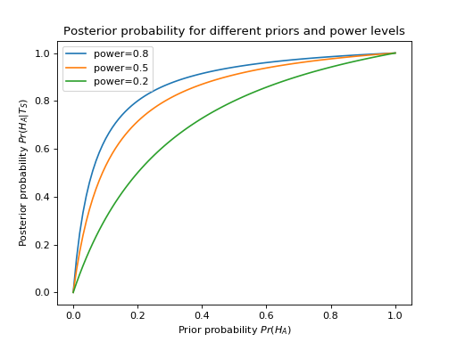
The posterior probability depends on the power. If the power is low and \(H_A\) is true, the likelihood of getting a significant test result is small. Assuming \(\pi = Pr(H_A) = 0.5\), our posterior probability is given by \(\Frac{(1 - \beta)}{(1 - \beta) + \alpha}\). As the chance of finding a true positive \(= 1-\beta\) drops towards the chance of finding a false negative \(= \alpha\), our confidence in the truth of the significant result must drop too.
The posterior likelihood also depends on the prior. When the prior \(Pr(H_A)\) drops then we become more wary of the (apriori more unlikely) true positive compared to the (apriori more likely) false positive.
As you can see from the figure. When power is 0.2, and the prior probability is less than around 0.2, then even if there is a significant test result, the null is still more likely than the \(H_A\) (posterior < 0.5).
Quantifying the effect of bias
Working scientists know that working scientists have many sources of bias in data collection and analysis.
We tend to assume that the effect of this bias is relatively minor. Is this true?
Ioannidis quantifies bias with a parameter \(u\). \(u\) is the proportion of not-significant findings that become significant as a result of bias. Put another way, the effect of bias is the result of taking the second column in the probability table above (the not-significant findings) and multiplying by \(u\). We add this effect to the first column (significant findings) and subtract from the second column (not-significant findings). Before applying the priors, this looks like:
>>> u = symbols('u')
>>> bias_assoc_noprior = dict(t_s = (1 - beta) + u * beta,
...                           t_ns = beta - u * beta,
...                           f_s = alpha + u * (1 - alpha),
...                           f_ns = (1 - alpha) - u * (1 - alpha))
\(\mathtt{\text{T\_S}}\) |
\(\mathtt{\text{T\_N}}\) |
|
\(H_A\) |
\(1 - \beta + \beta u\) |
\(\beta - \beta u\) |
\(H_0\) |
\(\alpha + u \left(1 - \alpha\right)\) |
\(1 - \alpha - u \left(1 - \alpha\right)\) |
Total |
\(1 + \alpha - \beta + \beta u + u \left(1 - \alpha\right)\) |
\(1 + \beta - \alpha - \beta u - u \left(1 - \alpha\right)\) |
After applying the prior:
>>> bias_assoc = bias_assoc_noprior.copy()
>>> bias_assoc['t_s'] *= pi
>>> bias_assoc['t_ns'] *= pi
>>> bias_assoc['f_s'] *= 1 - pi
>>> bias_assoc['f_ns'] *= 1 - pi
\(\mathtt{\text{T\_S}}\) |
\(\mathtt{\text{T\_N}}\) |
|
\(H_A\) |
\(\pi \left(1 - \beta + \beta u\right)\) |
\(\pi \left(\beta - \beta u\right)\) |
\(H_0\) |
\(\left(1 - \pi\right) \left(\alpha + u \left(1 - \alpha\right)\right)\) |
\(\left(1 - \pi\right) \left(1 - \alpha - u \left(1 - \alpha\right)\right)\) |
Total |
\(\pi \left(1 - \beta + \beta u\right) + \left(1 - \pi\right) \left(\alpha + u \left(1 - \alpha\right)\right)\) |
\(\pi \left(\beta - \beta u\right) + \left(1 - \pi\right) \left(1 - \alpha - u \left(1 - \alpha\right)\right)\) |
The first cell in the table is \(Pr(T_S | H_A) Pr(H_A)\). The total for the first column gives \(Pr(T_S)\). Therefore the posterior probability \(Pr(H_A | T_S)\) is:
>>> post_prob_bias = bias_assoc['t_s'] / (bias_assoc['t_s'] +
...                                       bias_assoc['f_s'])
>>> post_prob_bias
pi*(beta*u - beta + 1)/(pi*(beta*u - beta + 1) + (alpha + u*(-alpha + 1))*(-pi + 1))
>>> # Same as Ioannidis formulation?
>>> # This from Ioannidis 2005:
>>> ppv_bias = (
...     ((1 - beta) * R + u * beta * R) /
...     (R + alpha - beta * R + u - u * alpha + u * beta * R)
...    )
>>> # Is this the same as our formula above?
>>> simplify(ppv_bias - post_prob_bias) == 0
True
What effect does bias have on the posterior probabilities?
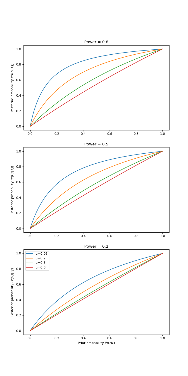
As we’d expect, as bias increases to 1, the result of the experiment has less and less effect on our posterior estimate. If the analysis was entirely biased, then our posterior estimate is unchanged from the prior (diagonal line on the graph).
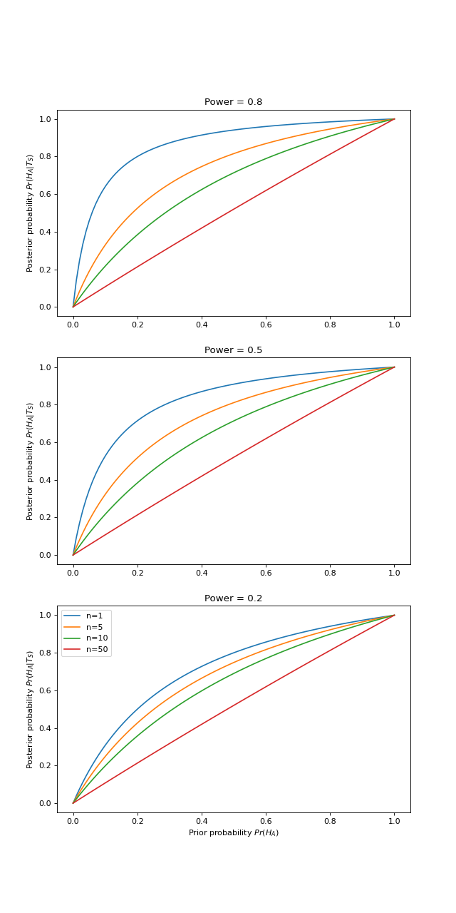
The effect of multiple studies
Ioannidis makes the point that when a field is particularly fashionable, there may be many research groups working on the same question.
Given publication bias for positive findings, it is possible that only positive research findings will be published. If \(n\) research groups have done the same experiment, then the probability that all the \(n\) studies will be not significant, given \(H_A\) is true, is \(\beta^n\). Conversely the probability that there is at least one positive finding in the \(n\) tests is \(1 - \beta^n\). Similarly the probability that all \(n\) studies will be not significant, given \(H_0\), is \((1 - \alpha)^n\). The probability of at least one false positive is \(1 - (1 - \alpha)^n\).
The probability table (without the priors) is:
>>> n = symbols('n')
>>> multi_assoc_noprior = dict(t_s = (1 - beta ** n),
...                           t_ns = beta ** n,
...                           f_s = 1 - (1 - alpha) ** n,
...                           f_ns = (1 - alpha) ** n)
\(\mathtt{\text{T\_S}}\) |
\(\mathtt{\text{T\_N}}\) |
|
\(H_A\) |
\(1 - \beta^{n}\) |
\(\beta^{n}\) |
\(H_0\) |
\(1 - \left(1 - \alpha\right)^{n}\) |
\(\left(1 - \alpha\right)^{n}\) |
Total |
\(2 - \beta^{n} - \left(1 - \alpha\right)^{n}\) |
\(\beta^{n} + \left(1 - \alpha\right)^{n}\) |
Considering the prior:
>>> multi_assoc = multi_assoc_noprior.copy()
>>> multi_assoc['t_s'] *= pi
>>> multi_assoc['t_ns'] *= pi
>>> multi_assoc['f_s'] *= 1 - pi
>>> multi_assoc['f_ns'] *= 1 - pi
\(\mathtt{\text{T\_S}}\) |
\(\mathtt{\text{T\_N}}\) |
|
\(H_A\) |
\(\pi \left(1 - \beta^{n}\right)\) |
\(\pi \beta^{n}\) |
\(H_0\) |
\(\left(1 - \pi\right) \left(1 - \left(1 - \alpha\right)^{n}\right)\) |
\(\left(1 - \alpha\right)^{n} \left(1 - \pi\right)\) |
Total |
\(\pi \left(1 - \beta^{n}\right) + \left(1 - \pi\right) \left(1 - \left(1 - \alpha\right)^{n}\right)\) |
\(\pi \beta^{n} + \left(1 - \alpha\right)^{n} \left(1 - \pi\right)\) |
Giving posterior probability of:
>>> post_prob_multi = multi_assoc['t_s'] / (multi_assoc['t_s'] + multi_assoc['f_s'])
>>> post_prob_multi
pi*(-beta**n + 1)/(pi*(-beta**n + 1) + (-pi + 1)*(-(-alpha + 1)**n + 1))
>>> # Formula from Ioannidis 2005:
>>> ppv_multi = R * (1 - beta ** n) / (R + 1 - (1 - alpha) ** n - R * beta ** n)
>>> # Is this the same as our formula above?
>>> simplify(ppv_multi - post_prob_multi) == 0
True
Putting it together
Considering analysis bias and positive publication bias together:
>>> multi_bias_assoc_noprior = dict(
...    t_s = (1 - beta ** n) + u * beta ** n,
...    t_ns = beta ** n - u * beta ** n,
...    f_s = 1 - (1 - alpha) ** n + u * (1 - alpha) ** n,
...    f_ns = (1 - alpha) ** n - u * (1 - alpha)**n)
\(\mathtt{\text{T\_S}}\) |
\(\mathtt{\text{T\_N}}\) |
|
\(H_A\) |
\(1 - \beta^{n} + u \beta^{n}\) |
\(\beta^{n} - u \beta^{n}\) |
\(H_0\) |
\(1 - \left(1 - \alpha\right)^{n} + u \left(1 - \alpha\right)^{n}\) |
\(\left(1 - \alpha\right)^{n} - u \left(1 - \alpha\right)^{n}\) |
Total |
\(2 - \beta^{n} - \left(1 - \alpha\right)^{n} + u \beta^{n} + u \left(1 - \alpha\right)^{n}\) |
\(\beta^{n} + \left(1 - \alpha\right)^{n} - u \beta^{n} - u \left(1 - \alpha\right)^{n}\) |
>>> multi_bias_assoc = multi_bias_assoc_noprior.copy()
>>> multi_bias_assoc['t_s'] *= pi
>>> multi_bias_assoc['t_ns'] *= pi
>>> multi_bias_assoc['f_s'] *= 1 - pi
>>> multi_bias_assoc['f_ns'] *= 1 - pi
\(\mathtt{\text{T\_S}}\) |
\(\mathtt{\text{T\_N}}\) |
|
\(H_A\) |
\(\pi \left(1 - \beta^{n} + u \beta^{n}\right)\) |
\(\pi \left(\beta^{n} - u \beta^{n}\right)\) |
\(H_0\) |
\(\left(1 - \pi\right) \left(1 - \left(1 - \alpha\right)^{n} + u \left(1 - \alpha\right)^{n}\right)\) |
\(\left(1 - \pi\right) \left(\left(1 - \alpha\right)^{n} - u \left(1 - \alpha\right)^{n}\right)\) |
Total |
\(\pi \left(1 - \beta^{n} + u \beta^{n}\right) + \left(1 - \pi\right) \left(1 - \left(1 - \alpha\right)^{n} + u \left(1 - \alpha\right)^{n}\right)\) |
\(\pi \left(\beta^{n} - u \beta^{n}\right) + \left(1 - \pi\right) \left(\left(1 - \alpha\right)^{n} - u \left(1 - \alpha\right)^{n}\right)\) |
>>> post_prob_multi_bias = (
...    multi_bias_assoc['t_s'] /
...    (multi_bias_assoc['t_s'] + multi_bias_assoc['f_s'])
...    )
>>> post_prob_multi_bias
pi*(beta**n*u - beta**n + 1)/(pi*(beta**n*u - beta**n + 1) + (-pi + 1)*(u*(-alpha + 1)**n - (-alpha + 1)**n + 1))
Now we make a numerical version of this symbolic expression, so we can evaluate it for different values of \(\alpha, \beta, \pi, u, n\):
>>> # Make numerical version of symbolic expression
>>> pp_mb_func = lambdify((alpha, beta, pi, u, n), post_prob_multi_bias)
Let’s assume that two groups are doing more or less the same study, and only the positive study publishes (\(n = 2\)). There is an analysis bias of 10% (\(u= 0.1\)). We take the power from the Button et al estimate for neuroimaging studies = 0.08. Therefore \(\beta = 1 - 0.08 = 0.92\):
Button, Katherine S., John PA Ioannidis, Claire Mokrysz, Brian A. Nosek, Jonathan Flint, Emma SJ Robinson, and Marcus R. Munafò. 2013. “Power failure: why small sample size undermines the reliability of neuroscience.” Nature Reviews Neuroscience.
This graph tells us that, for a study with average power in neuroimaging, with some mild analysis bias and positive publication bias, the significant finding \(T_S\) does not change our posterior very much from our prior.
If we do some study with an hypothesis that is suitably unlikely apriori - say \(Pr(H_A) = 0.25\) - then our posterior probability is:
>>> print(pp_mb_func(0.05, 0.92, 0.25, 0.1, 2))
0.2972463786...
What if the result was significant at \(p < 0.01\)?:
>>> print(pp_mb_func(0.01, 0.92, 0.25, 0.1, 2))
0.40245282700...
So, even if our result is significant at \(p < 0.01\), the probability that \(H_A\) is correct is still less than \(0.5\).