\(\newcommand{L}[1]{\| #1 \|}\newcommand{VL}[1]{\L{ \vec{#1} }}\newcommand{R}[1]{\operatorname{Re}\,(#1)}\newcommand{I}[1]{\operatorname{Im}\, (#1)}\)

The Fourier basis

Fourier without the ei shows that we can write the discrete Fourier transform DFT as vector dot products. In Rewriting the DFT with vectors we found that:

\[X_k = \vec{x} \cdot \vec{c^k} - i \vec{x} \cdot \vec{s^k}\]

where:

\[\begin{split}\vec{r^k} = [ k 2 \pi \frac{0}{N}, k 2 \pi \frac{1}{N}, k 2 \pi \frac{N-1}{N}] \\ \vec{c^k} \triangleq \left[ \cos(r^k_0), \cos(r^k_1), \ldots \cos(r^k_{N-1} \right] \\ \vec{s^k} \triangleq \left[ \sin(r^k_0), \sin(r^k_1), \ldots \sin(r^k_{N-1} \right]\end{split}\]

\(\vec{c_k}, \vec{s_k}\) are Fourier basis vectors.

We can compile all these vectors into matrices to form Fourier basis matrices.

Rewriting the DFT with cosine and sine basis matrices

Instead of writing the formulae for the individual elements \(X_k\) and \(x_n\), we can use matrices to express our formulae in terms of the vectors \(\vec{X}, \vec{x}\).

\(\newcommand{C}{\mathbf{C}} \newcommand{S}{\mathbf{S}}\) Define a matrix \(\C\) that has rows \([\vec{c_0}, \vec{c_1}, ..., \vec{c_{N-1}}]\):

\[\begin{split}\C \triangleq \begin{bmatrix} c_{0,0}, c_{0, 1}, ..., c_{0, N-1} \\ c_{1,0}, c_{1, 1}, ..., c_{1, N-1} \\ ... \\ c_{N-1,0}, c_{N-1, 1}, ..., c_{N-1, N-1} \\ \end{bmatrix}\end{split}\]

Call \(\C\) the cosine basis matrix.

Define a matrix \(\S\) that has rows \([\vec{s_0}, \vec{s_1}, ..., \vec{s_{N-1}}]\):

\[\begin{split}\S \triangleq \begin{bmatrix} s_{0,0}, s_{0, 1}, ..., s_{0, N-1} \\ s_{1,0}, s_{1, 1}, ..., s_{1, N-1} \\ ... \\ s_{N-1,0}, s_{N-1, 1}, ..., s_{N-1, N-1} \\ \end{bmatrix}\end{split}\]

Call \(\S\) the sine basis matrix.

Now we can rewrite the forward and inverse DFT as matrix products:

\[\begin{split}\vec{X} = \C \cdot \vec{x} - i \S \cdot \vec{x} \\ \vec{x} = \frac{1}{N} \C \cdot \vec{X} + i \frac{1}{N} \S \cdot \vec{X}\end{split}\]

Loading display libraries and data

>>> import numpy as np
>>> np.set_printoptions(precision=4, suppress=True)
>>> x = np.array(
...     [ 0.4967, -0.1383,  0.6477,  1.523 , -0.2342, -0.2341,  1.5792,
...       0.7674, -0.4695,  0.5426, -0.4634, -0.4657,  0.242 , -1.9133,
...      -1.7249, -0.5623, -1.0128,  0.3142, -0.908 , -1.4123,  1.4656,
...      -0.2258,  0.0675, -1.4247, -0.5444,  0.1109, -1.151 ,  0.3757,
...      -0.6006, -0.2917, -0.6017,  1.8523])
>>> N = len(x)

In order to run the commands in this page, you will need to download the file dft_plots.py to the directory where you running the code.

>>> import matplotlib.pyplot as plt
>>> import dft_plots as dftp

Hint

If running in the IPython console, consider running %matplotlib to enable interactive plots. If running in the Jupyter Notebook, use %matplotlib inline.

Some properties of the cosine and sine basis matrices

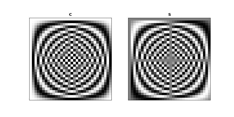
First we note that \(\C\) and \(\S\) are always real matrices, regardless of the input \(\vec{x}\) or \(\vec{X}\).

Let’s show \(\C\) and \(\S\) as grayscale images.

First we build \(\C\) and \(\S\) for our case with \(N=32\):

>>> C = np.zeros((N, N))
>>> S = np.zeros((N, N))
>>> ns = np.arange(N)
>>> one_cycle = 2 * np.pi * ns / N
>>> for k in range(N):
...     t_k = k * one_cycle
...     C[k, :] = np.cos(t_k)
...     S[k, :] = np.sin(t_k)

>>> fig, axes = plt.subplots(1, 2, figsize=(10, 5))
>>> dftp.show_array(axes[0], dftp.scale_array(C))
>>> axes[0].set_title("$\mathbf{C}$")
<...>
>>> dftp.show_array(axes[1], dftp.scale_array(S))
>>> axes[1].set_title("$\mathbf{S}$")
<...>

(png, hires.png, pdf)

Mirror symmetry

From the images we see that the bottom half of \(\C\) looks like a mirror image of the top half of \(\C\). The bottom half of \(\S\) looks like a sign flipped (black \(\Leftrightarrow\) white) mirror image of the top half of \(\S\). In fact this is correct:

\[\begin{split}C_{p,:} = C_{N-p,:} \; \mathrm{for} \; p > 0 \\ S_{p,:} = -S_{N-p,:} \; \mathrm{for} \; p > 0\end{split}\]

Why is this? Let’s look at lines from the center of \(\C\). Here we are plotting the continuous cosine function with dotted lines, with filled circles to represent the discrete samples we took to fill the row of \(\C\):

>>> center_rows = [N / 2. - 1, N / 2., N / 2. + 1]
>>> fig = dftp.plot_cs_rows('C', N, center_rows)
>>> fig.suptitle('Rows $N / 2 - 1$ through $N / 2 + 1$ of $\mathbf{C}$',
...              fontsize=20)
<...>

(png, hires.png, pdf)

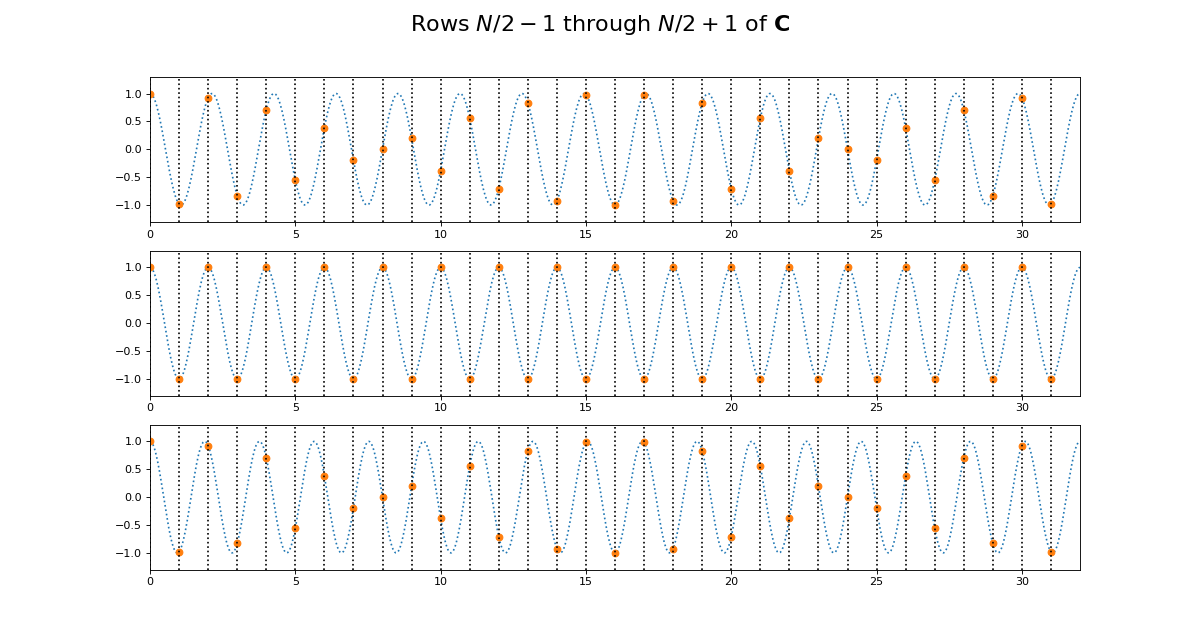
The first plot in this grid is for row \(k = N / 2 - 1\). This row starts sampling just before the peak and trough of the cosine. In the center is row \(k = N / 2\) of \(\C\). This is sampling the cosine wave exactly at the peak and trough. When we get to next row, at \(k = N / 2 + 1\), we start sampling after the peak and trough of the cosine, and these samples are identical to the samples just before the peak and trough, at row \(k = N / 2 - 1\). Row \(k = N / 2\) is sampling at the Nyquist sampling frequency, and row \(k = N / 2 + 1\) is sampling at a frequency lower than Nyquist and therefore it is being aliased to the same apparent frequency as row \(k = N / 2 - 1\).

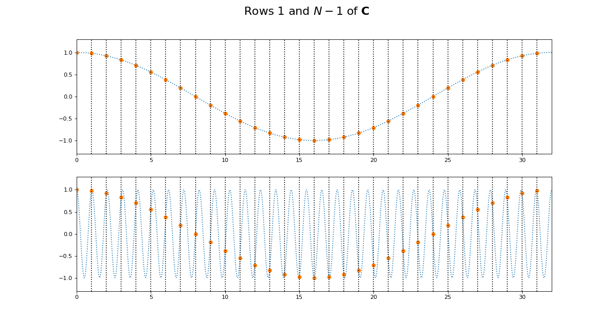
This might be more obvious plotting rows 1 and N-1 of \(\C\):

>>> fig = dftp.plot_cs_rows('C', N, [1, N-1])
>>> fig.suptitle('Rows $1$ and $N - 1$ of $\mathbf{C}$',
...              fontsize=20)
<...>

(png, hires.png, pdf)

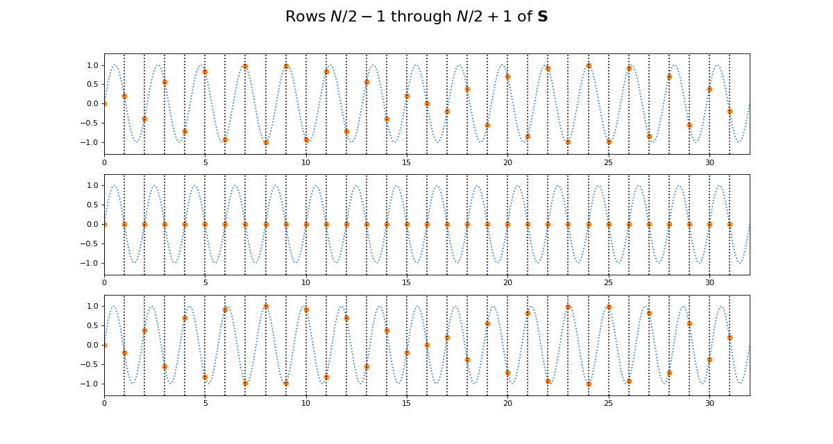
Of course we get the same kind of effect for \(\S\):

>>> fig = dftp.plot_cs_rows('S', N, center_rows)
>>> fig.suptitle('Rows $N / 2 - 1$ through $N / 2 + 1$ of $\mathbf{S}$',
...              fontsize=20)
<...>

(png, hires.png, pdf)

>>> fig = dftp.plot_cs_rows('S', N, [1, N-1])
>>> fig.suptitle('Rows $1$ and $N - 1$ of $\mathbf{S}$',
...              fontsize=20)
<...>

(png, hires.png, pdf)

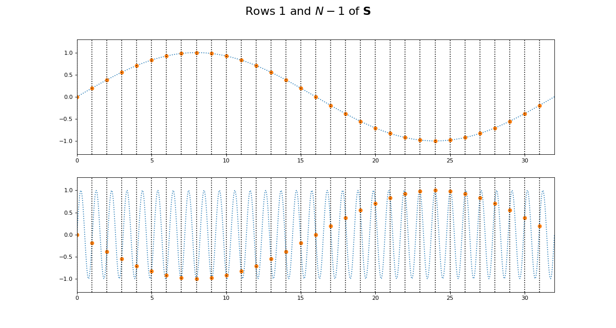
Notice that for \(\S\), the sine waves after \(k = N / 2\) are sign-flipped relative to their matching rows before \(k = N / 2\). Thus row \(k = N / 2 + 1\) will be aliased to the same frequency as for row \(k = N / 2 - 1\), but with a negative sign.

It is this sign-flip that leads to the concept of negative frequency in the DFT, and to the property of conjugate symmetry from the DFT on a vector of real numbers. We will hear more about these later.

Matrix symmetry

The next thing we notice about \(\C\) and \(\S\) is that they are transpose symmetric matrices:

\[\begin{split}\C = \C^T \\ \S = \S^T \\\end{split}\]

>>> assert np.allclose(C, C.T)
>>> assert np.allclose(S, S.T)

Why is this? Consider the first column of \(\C\). This is given by \(\cos(k 2 \pi 0 / N) = \cos(0)\), and thus, like the first row of \(\C\), is always = 1.

Now consider the second row of \(\C\). This is a cosine sampled at horizontal axis values:

\[\vec{t_1} \triangleq \left[ 2 \pi \frac{n}{N} \;\mathrm{for}\; n \in 0,1,\ldots,N-1 \right]\]

Call \(t_{k, n}\) the value of \(\vec{t_k}\) at index \(n\). Now consider the second column of \(\C\). This is a cosine sampled at horizontal axis values for \(n = 1\):

\[\begin{split}t_{0,1} = (0) 2 \pi \frac{1}{N} \\ t_{1,1} = (1) 2 \pi \frac{1}{N} \\ ... \\ t_{N-1,1} = (N-1) 2 \pi \frac{1}{N} \\\end{split}\]

In general, because the sequence \(k 0,1,,N-1 \) is equal to the sequence \(n \in 0,1,\ldots,N-1\), this means that the column sampling positions for row \(n \in t_{0, n}, t_{1, n}, ... , t_{N-1, n}\) are equal to the row sampling positions for corresponding (\(k = n\)) row \(k \in t_{k, 0}, t_{k, 1}, ... , t_{k, N-1}\). Write column \(z\) of \(\C\) as \(C_{:,z}\); column \(z\) of \(\S\) is \(S_{:, z}\). Therefore \(C_{z, :} = C_{:, z}, S_{z, :} = S_{:, z}\).

Row dot products and lengths

It is useful to look at the dot products of the rows of \(\C\) and \(\S\). The dot product of each row with itself gives the squared length of the vector in that row.

The vector length of a vector \(\vec{v}\) with \(N\) elements is written as \(\| \vec{v} \|\), and defined as:

\[\| \vec{v} \| \triangleq \sqrt{\sum_{n=0}^{N-1} v_n^2} = \sqrt{ \vec{v} \cdot \vec{v} }\]

The dot products of different rows of \(\C\) and \(\S\) give an index of the strength of the relationship between the rows. We can look at the dot products of all the rows of \(\C\) with all other rows with the matrix multiplication \(\C^T \C\):

>>> dftp.show_array(plt.gca(), dftp.scale_array(C.T.dot(C)))
>>> plt.title("$\mathbf{C^TC}$")
<...>

(png, hires.png, pdf)

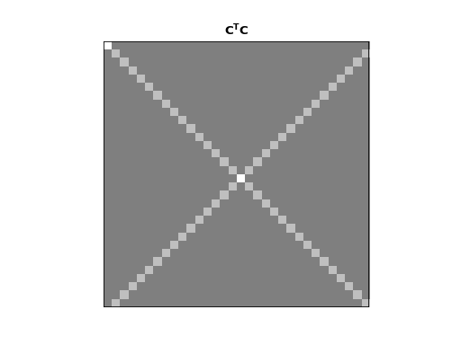
The image shows us that the dot product between the rows of \(\C\) is 0 everywhere except:

• the dot products of the rows with themselves (the squared vector lengths);
• the dot products of the mirror image vectors such as \(\vec{c_1}\) and \(\vec{c_{N-1}}\). Because \(\vec{c_n} = \vec{c_{N-n}}\), these dot products are the same as the \(\| \vec{c_n} \|^2\).

The squared row lengths are:

>>> np.diag(C.T.dot(C))
array([ 32.,  16.,  16.,  16.,  16.,  16.,  16.,  16.,  16.,  16.,  16.,
        16.,  16.,  16.,  16.,  16.,  32.,  16.,  16.,  16.,  16.,  16.,
        16.,  16.,  16.,  16.,  16.,  16.,  16.,  16.,  16.,  16.])

Notice that the rows \(\vec{c_0}\) and \(\vec{c_{N / 2}}\) have squared length \(N\), and the other rows have squared length \(N / 2\).

We can do the same for \(\S\):

>>> dftp.show_array(plt.gca(), dftp.scale_array(S.T.dot(S)))
>>> plt.title("$\mathbf{S^TS}$")
<...>

(png, hires.png, pdf)

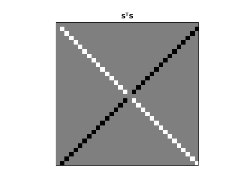
Remember that \(\vec{s_0}\) and \(\vec{s_{n/2}}\) are all 0 vectors. The dot product of these rows with any other row, including themselves, is 0. All other entries in this \(\S^T \S\) matrix are zero except:

• the dot products of rows with themselves (other than \(\vec{s_0}\) and \(\vec{s_{n/2}}\));
• the dot products of the flipped mirror image vectors such as \(\vec{s_1}\) and \(\vec{s_{N-1}}\). Because \(\vec{s_n} = -\vec{s_{N-n}}\), these dot products are the same as \(-\| \vec{s_n} \|^2\).

The squared row lengths are:

>>> np.diag(S.T.dot(S))
array([  0.,  16.,  16.,  16.,  16.,  16.,  16.,  16.,  16.,  16.,  16.,
        16.,  16.,  16.,  16.,  16.,   0.,  16.,  16.,  16.,  16.,  16.,
        16.,  16.,  16.,  16.,  16.,  16.,  16.,  16.,  16.,  16.])

The rows \(\vec{s_0}\) and \(\vec{s_{N / 2}}\) have squared length \(0\), and the other rows have squared length \(N / 2\).

Finally, let’s look at the relationship between the rows of \(\C\) and the rows of \(\S\):

>>> np.allclose(C.T.dot(S), 0)
True

The rows of \(\C\) and \(\S\) are completely orthogonal.

In fact these relationships hold for \(\C\) and \(\S\) for any \(N\).

Proof for \(\C, \S\) dot products

We can show these relationships with some more or less basic trigonometry.

Let’s start by looking at the dot product of two rows from \(\C\). We will take rows \(\vec{c_p} =\C_{p,:}\) and \(\vec{c_q} = \C_{q,:}\). As we remember, these vectors are:

\[\begin{split}\vec{c_p} = \left[ \cos(p n \frac{2 \pi}{N}) \;\mathrm{for}\; n \in 0,1,\ldots,N-1 \right] \\ \vec{c_q} = \left[ \cos(q n \frac{2 \pi}{N}) \;\mathrm{for}\; n \in 0,1,\ldots,N-1 \right]\end{split}\]

So:

\[\vec{c_p} \cdot \vec{c_q} = \sum_{n=0}^{N-1} \cos(p n \frac{2 \pi}{N}) \cos(q n \frac{2 \pi}{N})\]

Our trigonometry tells us that:

\[\cos \alpha \cos \beta = \frac{1}{2} [ \cos(\alpha + \beta) - \cos(\alpha - \beta) ]\]

We can rewrite the dot product as the addition of two sums of cosines:

\[\vec{c_p} \cdot \vec{c_q} = \frac{1}{2} \sum_{n=0}^{N-1} \cos((p + q) n \frac{2 \pi}{N}) + \frac{1}{2} \sum_{n=0}^{N-1} \cos((p - q) n \frac{2 \pi}{N})\]

Now we can use the formulae for sums of arithmetic progressions of cosines and sines to solve these equations. Here are the formulae:

\[\begin{split}R \triangleq \frac{\sin(N \frac{1}{2}d)}{\sin(\frac{1}{2} d)} \\ \sum_{n=0}^{N-1} \cos(a + nd) = \begin{cases} N \cos a & \text{if } \sin(\frac{1}{2}d) = 0 \\ R \cos ( a + (N - 1) \frac{1}{2} d) & \text{otherwise} \end{cases} \\ \sum_{n=0}^{N-1} \sin(a + nd) = \begin{cases} N \sin a & \text{if } \sin(\frac{1}{2}d) = 0 \\ R \sin ( a + (N - 1) \frac{1}{2} d) & \text{otherwise} \end{cases}\end{split}\]

For our \(\C, \S\) row dot product sums, starting angle \(a\) is always 0, and the \(d\) value in the formulae are always integer multiples of \(\frac{2 \pi}{N}\). For example, \(d = (p \pm q) \frac{2 \pi}{N}\) in the equations above. For our case, we can write \(d = g \frac{2 \pi}{N}\) where \(g\) is an integer.

\[\begin{split}R = \frac{ \sin( g N \frac{1}{2} \frac{2 \pi}{N} ) } { \sin( g \frac{1}{2} \frac{2 \pi}{N} ) } \\ = \frac{ \sin( g \pi ) } { \sin( \frac{g}{N} \pi ) }\end{split}\]

Because \(g\) is an integer, the numerator of \(R\) will always be 0, so the resulting sum is zero unless the denominator of \(R\) is zero. The denominator is zero only if \(g\) is a multiple of N, including 0. When the denominator is zero, the sum will be equal to \(N \cos(a) = N \cos(0) = N\) for a cosine series or \(N \sin(a) = N \sin(0) = 0\) for a sine series.

Now we can calculate our dot product:

\[\begin{split}\vec{c_p} \cdot \vec{c_q} = \begin{cases} \frac{1}{2} N + \frac{1}{2} N = N & \text{if } p = q, p \in 0, N/2 \\ \frac{1}{2} N & \text{if } p = q, p \notin 0, N/2 \\ \frac{1}{2} N & \text{if } p + q = N, p \ne N/2 \\ 0 & \text{otherwise} \end{cases}\end{split}\]

We can apply the same kind of logic to the rows of \(\S\):

\[\sin \alpha \sin \beta = \frac{1}{2} [ \cos(\alpha - \beta) - \cos(\alpha + \beta) ]\]

So:

\[\vec{s_p} \cdot \vec{s_q} = \frac{1}{2} \sum_{n=0}^{N-1} \cos((p - q) n \frac{2 \pi}{N}) - \frac{1}{2} \sum_{n=0}^{N-1} \cos((p + q) n \frac{2 \pi}{N})\]

This gives:

\[\begin{split}\vec{s_p} \cdot \vec{s_q} = \begin{cases} 0 & \text{if } p = q, p \in 0, N/2 \\ \frac{1}{2} N & \text{if } p = q, p \notin 0, N/2 \\ -\frac{1}{2} N & \text{if } p + q = N, p \ne N/2 \\ 0 & \text{otherwise} \end{cases}\end{split}\]

• Download this page as a Python code file;
• Download this page as a Jupyter notebook (no outputs).