\(\newcommand{L}[1]{\| #1 \|}\newcommand{VL}[1]{\L{ \vec{#1} }}\newcommand{R}[1]{\operatorname{Re}\,(#1)}\newcommand{I}[1]{\operatorname{Im}\, (#1)}\)

Smoothing as convolution

We load and configure the libraries we need:

>>> # Import numerical and plotting libraries
>>> import numpy as np
>>> import numpy.linalg as npl
>>> import matplotlib.pyplot as plt

Hint

If running in the IPython console, consider running %matplotlib to enable interactive plots. If running in the Jupyter Notebook, use %matplotlib inline.

Smoothing as weighted average

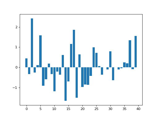
In the introduction to smoothing tutorial, we had the following random data:

>>> np.random.seed(5) # To get predictable random numbers
>>> n_points = 40
>>> x_vals = np.arange(n_points)
>>> y_vals = np.random.normal(size=n_points)
>>> plt.bar(x_vals, y_vals)
<...>

(png, hires.png, pdf)

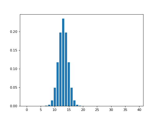
In the example, we generated a Gaussian kernel over the x axis at index 13. The kernel had a full-width-at-half-maximum value of 4. This corresponds to a Gaussian sigma value of about 1.7:

>>> def fwhm2sigma(fwhm):
...     return fwhm / np.sqrt(8 * np.log(2))

>>> sigma = fwhm2sigma(4)
>>> sigma
1.6986436005760381

>>> x_position = 13
>>> # Make Gaussian centered at 13 with given sigma
>>> kernel_at_pos = np.exp(-(x_vals - x_position) ** 2 / (2 * sigma ** 2))
>>> # Make kernel sum to 1
>>> kernel_at_pos = kernel_at_pos / sum(kernel_at_pos)
>>> plt.bar(x_vals, kernel_at_pos)
<...>

(png, hires.png, pdf)

The new smoothed value for x=13 is the sum of the data y values (\(y_i : i \in 0, 1, .. 39\)) multiplied by their respective kernel y values (\(k_i : i \in 0, 1, .. 39\)):

\[y_{13} = \sum _{i=0} ^{i=39} y_i k_i\]

>>> print(np.sum(y_vals * kernel_at_pos))
-0.347968590118

Of course this is also the dot product of the two vectors:

>>> print(y_vals.dot(kernel_at_pos))
-0.347968590118

Using a finite width for the kernel

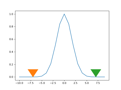
Looking at the plot of the kernel, it looks like we have many zero values, far from the central x=13 point. Maybe we could be more efficient, by only doing the y value multiplication for kernel values that are larger than some threshold, like 0.0001.

Let’s have another look at the Gaussian

>>> # Make a +/- x range large enough to let kernel drop to zero
>>> x_for_kernel = np.arange(-10, 10)
>>> # Calculate kernel
>>> kernel = np.exp(-(x_for_kernel) ** 2 / (2 * sigma ** 2))
>>> # Threshold
>>> kernel_above_thresh = kernel > 0.0001
>>> # Find x values where kernel is above threshold
>>> x_within_thresh = x_for_kernel[kernel_above_thresh]
>>> plt.plot(x_for_kernel, kernel)
[...]
>>> plt.plot(min(x_within_thresh), 0, marker=7, markersize=40)
[...]
>>> plt.plot(max(x_within_thresh), 0, marker=7, markersize=40)
[...]

(png, hires.png, pdf)

We can make a new kernel, with finite width, where the near-zero values have been trimmed:

>>> finite_kernel = kernel[kernel_above_thresh]
>>> # Make kernel sum to 1 again
>>> finite_kernel = finite_kernel / finite_kernel.sum()
>>> plt.plot(x_within_thresh, finite_kernel)
[...]

(png, hires.png, pdf)

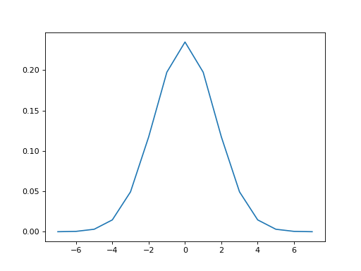
This kernel has a finite width:

>>> len(finite_kernel)
15

To get our smoothed value for x=13, we can shift this trimmed kernel be centered over x=13, and only multiply by the y values that are within the kernel width:

>>> # Number of kernel points before center (at 0)
>>> kernel_n_below_0 = int((len(finite_kernel) - 1) / 2.)
>>> kernel_n_below_0
7

Because we cut the kernel at a low threshold, the result from using the finite kernel is very similar to using the infinite kernel that we used above:

>>> # Multiply and sum y values within the finite kernel
>>> kernel_starts_at = 13 - kernel_n_below_0
>>> y_within_kernel = y_vals[kernel_starts_at : kernel_starts_at + len(finite_kernel)]
>>> print(np.dot(finite_kernel, y_within_kernel))
-0.347973672994

Smoothing as convolution

If are you familiar with convolution the smoothing procedure may be familiar.

With convolution, we also have a kernel, and we also generate values by taking the sum of the products of values within the kernel.

With convolution, we reverse the convolution kernel and the step through the y values, cross-multiplying the y signal with the reversed kernel.

That could work here too. There is no need for us to reverse the kernel, because it is symmetrical.

In fact, it might be possible to see that, we can get exactly our required result for x=13, by convolving the y values with the finite smoothing kernel.

>>> convolved_y = np.convolve(y_vals, finite_kernel)
>>> print(convolved_y[13+ kernel_n_below_0])
-0.347973672994

Why have I printed out the value at 13 + kernel_n_below_0 ? Because this is the convolution value that corresponds to the weighted sum we did with our original multiplication. When the convolution algorithm gets to this index, it applies the reversed smoothing kernel to this index and the len(finite_kernel) - 1 values before it. This is the exact same set of multiplications we did for the original multiplication. Thus, in order to get the same smoothed values as we did when we were multiplying by a centered kernel, we have to get the values from the convolved output from half the kernel width ahead of the index we are interested in.

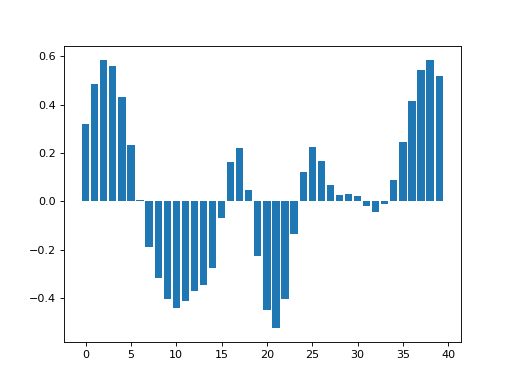
>>> smoothed_by_convolving = convolved_y[kernel_n_below_0:(n_points+kernel_n_below_0)]
>>> plt.bar(x_vals, smoothed_by_convolving)
<...>

(png, hires.png, pdf)

Here we were able to get the effect of an offset in the kernel, by taking an offset (kernel_n_below_0) in the output data. We have made use of the translation invariance property of convolution.

Convolution and edges

If you were very observant, you may have noticed that the convolution results above differ slightly from the convolution using the simple crude method in the An introduction to smoothing.

Here are those results for comparison:

>>> smoothed_vals = np.zeros(y_vals.shape)
>>> for x_position in x_vals:
...      kernel = np.exp(-(x_vals - x_position) ** 2 / (2 * sigma ** 2))
...      kernel = kernel / sum(kernel)
...      smoothed_vals[x_position] = sum(y_vals * kernel)
>>> plt.bar(x_vals, smoothed_vals)
<...>

(png, hires.png, pdf)

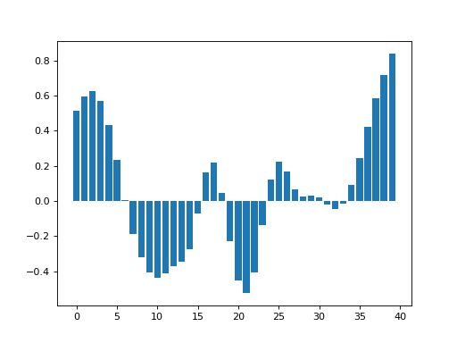
Notice that this plot has higher values at the edges of the data.

The reason is that the simple method above only evaluates the kernel for the x points present in the data. Therefore, at the left and right edges, this method is only applying half a Gaussian to the data. On the left it is applying the right half of the Gaussian, and on the right it is applying the left half of the Gaussian. Notice too that this simple method always makes the kernel sum to zero, so, when smoothing the points at the edges, with the half kernel, the remaining points get more weight.

This is one technique for dealing with the edges called truncating the kernel.

Convolution, by default, does not truncate the kernel, but assumes that data outside the x points we have are all zero. This is called zero padding. Using zero padding, the points towards the edge get pulled down towards zero because they are part-made of the result of taking the product of zero with the kernel values.

When we do spatial smoothing, this can be a significant problem. For example, imagine smoothing close to the bottom (inferior) edge of a brain image, where the edge voxels are likely to have brain signal. If we use zero padding then the values near the edge will get pulled towards zero causing a strong signal change from smoothing.

In this case we might prefer some other method of dealing with the data off the edge of the image, for example by assuming the signal is a flipped version of the signal going towards the edge. See the description of the mode argument in the docstring for scipy.ndimage.gaussian_filter for some other options.

• Download this page as a Python code file;

• Download this page as a Jupyter notebook (no outputs).