\(\newcommand{L}[1]{\| #1 \|}\newcommand{VL}[1]{\L{ \vec{#1} }}\newcommand{R}[1]{\operatorname{Re}\,(#1)}\newcommand{I}[1]{\operatorname{Im}\, (#1)}\)

Finding the least-squares line

Here I am using the matrix formulation of the linear model. See Introduction to the general linear model.

In general, if we have a design matrix \(X\) with columns of predictors, and a data vector \(\vec{y}\), then the least-squares fit of parameters for the columns of \(X\) is given by:

\[B = X^+ \vec{y}\]

\(X^+\) is called the pseudo-inverse of the design matrix \(X\).

When \(X^T X\) is invertible:

\[X^+ = (X^T X)^{-1} X^T\]

Here we are thinking about simple regression, where the design matrix has two columns. The first (say) is a column of 1s, modeling the intercept of the fitted line. The second contains an explanatory covariate, \(\vec{x}\).

\(X\) is dimension \(n\) rows, 2 columns.

As long as \(\vec{x}\) is not a constant, and therefore has more than one unique value, \(\vec{x}\) is not dependent on the column of 1s, and \(X^T X\) is invertible.

When the first column is the column of 1s, modeling the intercept, then the first row of \(B\) is the least-squares intercept, and the second row of \(B\) is the least-squares slope. Call that value \(B_2\).

Our desire is to be able to calculate \(B_2\) without doing anything nasty like not-trivial matrix inversion.

This requires that \(X^T X\) is a diagonal matrix, so we can invert it by dividing its diagonal elements into 1.

In order for this to work, the columns of \(X\) must be orthogonal. Therefore the covariate \(\vec{x}\), and therefore the second column of \(X\), must have zero mean. In that case:

\[\begin{split}X^T X = \begin{bmatrix} n & 0 \\ 0 & \sum{x_i^2} \end{bmatrix}\end{split}\]

From the inverse of a diagonal matrix.

\[\begin{split}(X^T X)^{-1} = \begin{bmatrix} \frac{1}{n} & 0 \\ 0 & \frac{1}{\sum{x_i^2}} \end{bmatrix}\end{split}\]

For neatness, let:

\[d = \frac{1}{\sum{x_i^2}}\]

\[\begin{split}(X^T X)^{-1} X^T = \begin{bmatrix} \frac{1}{n} & \frac{1}{n} & \dots & \frac{1}{n} \\ d x_1 & d x_2 & \dots & d x_n \end{bmatrix}\end{split}\]

\[\begin{split}(X^T X)^{-1} X^T \vec{y} = \begin{bmatrix} \frac{1}{n} \sum{y_i} \\ d \sum{x_i y_i} \end{bmatrix}\end{split}\]

This implies, for any not-constant covariate \(\vec{x}\) of mean 0, the intercept is at the mean of \(\vec{y}\), and the slope is:

\[\frac{\sum{x_i y_i}}{\sum{x_i^2}}\]

Now consider a covariate \(\vec{x}\) that does not have zero mean.

Adding or subtracting a constant to \(\vec{x}\) moves the data to the left and right on the x axis, and therefore changes the intercept of a best fit line, but it does not change the slope of this line.

For any covariate \(\vec{x}\), first calculate the mean; call this \(\bar{x}\). Call the mean of \(\vec{y}\): \(\bar{y}\). Subtract \(\bar{x}\) from every value in \(\vec{x}\) to give \(\vec{x_m}\). Find the slope and intercept for the best fit line of \(\vec{x_m}\) to \(\vec{y}\) as above. Adding back the mean will translate the line on the x axis such that \(x=0\) becomes \(x=\bar{x}\). The \(\vec{x_m}\) intercept is \(x=0, y=\bar{y}\). After translation, this point is at \(x=\bar{x}\), \(y=\bar{y}\). Given this point, and the slope, \(s\), the new intercept is \(\bar{y} - s \bar{x}\).

In action

Here we try the technique above with some simulated data.

Start with our usual imports:

>>> import numpy as np
>>> np.set_printoptions(precision=2, suppress=True)
>>> np.random.seed(5) # To get predictable random numbers
>>> import matplotlib.pyplot as plt

Hint

If running in the IPython console, consider running %matplotlib to enable interactive plots. If running in the Jupyter Notebook, use %matplotlib inline.

Here are random numbers to simulate \(\vec{x}\) and \(\vec{y}\).

>>> n = 20
>>> # Values from normal distribution with mean 18, SD 2.
>>> x = np.random.normal(18, 2, size=n)
>>> # Values from normal distribution with mean 10, SD 1.
>>> # Add half of x, to give linear relationship.
>>> y = np.random.normal(10, 1, size=n) * x / 2

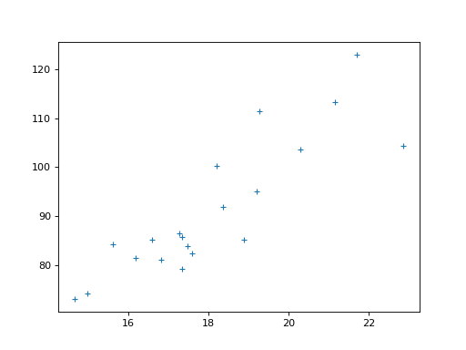
Plot simulated x and y:

>>> plt.plot(x, y, '+')
[...]

(png, hires.png, pdf)

Make the design matrix for the full linear model estimation:

>>> X = np.ones((n, 2))
>>> X[:, 1] = x

Do full linear model least-squares estimation. The first value in B is the intercept, the second is the slope.

>>> B = np.linalg.pinv(X) @ y
>>> B
array([-7.70,  5.47])

Now apply the algorithm above, to find the least-squares intercept and slope.

>>> def get_line(x, y):
...     x_bar = np.mean(x)
...     x_m = x - x_bar
...     slope = np.sum(x_m * y) / np.sum(x_m * x_m)
...     inter = np.mean(y) - slope * x_bar
...     return inter, slope

We get the same values as for the full estimation:

>>> get_line(x, y)
(-7.70217142823428, 5.467095969771854)