\(\newcommand{L}[1]{\| #1 \|}\newcommand{VL}[1]{\L{ \vec{#1} }}\newcommand{R}[1]{\operatorname{Re}\,(#1)}\newcommand{I}[1]{\operatorname{Im}\, (#1)}\)
Matrix rank
The rank of a matrix is the number of independent rows and / or columns of a matrix.
We will soon define what we mean by the word independent.
For a matrix with more columns than rows, it is the number of independent rows.
For a matrix with more rows than columns, like a design matrix, it is the number of independent columns.
In fact, linear algebra tells us that it is impossible to have more independent columns than there are rows, or more independent rows than there are columns. Try it with some test matrices.
A column is dependent on other columns if the values in the column can be generated by a weighted sum of one or more other columns.
To put this more formally - let’s say we have a matrix \(\mathbf{X}\) with \(M\) rows and \(N\) columns. Write column \(i\) of \(\mathbf{X}\) as \(X_{:,i}\). Column \(i\) is independent of the rest of \(\mathbf{X}\) if there is no length \(N\) column vector of weights \(\vec{c}\), where \(c_i = 0\), such that \(\mathbf{X} \cdot \vec{c} = X_{:,i}\).
Let’s make a design with independent columns:
>>> #: Standard imports
>>> import numpy as np
>>> # Make numpy print 4 significant digits for prettiness
>>> np.set_printoptions(precision=4, suppress=True)
>>> import matplotlib.pyplot as plt
>>> # Default to nearest neighbor interpolation, gray colormap
>>> import matplotlib
>>> matplotlib.rcParams['image.interpolation'] = 'nearest'
>>> matplotlib.rcParams['image.cmap'] = 'gray'
Hint
If running in the IPython console, consider running %matplotlib to enable
interactive plots. If running in the Jupyter Notebook, use %matplotlib
inline.
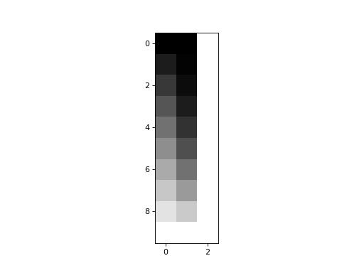
>>> trend = np.linspace(0, 1, 10)
>>> X = np.ones((10, 3))
>>> X[:, 0] = trend
>>> X[:, 1] = trend ** 2
>>> plt.imshow(X)
<...>

In this case, no column can be generated by a weighted sum of the other two.
We can test this with np.linalg.matrix_rank:
>>> import numpy.linalg as npl
>>> npl.matrix_rank(X)
3
This does not mean the columns are orthogonal:
>>> # Orthogonal columns have dot products of zero
>>> X.T.dot(X)
array([[  3.5185,   2.7778,   5.    ],
       [  2.7778,   2.337 ,   3.5185],
       [  5.    ,   3.5185,  10.    ]])
Nor does it mean that the columns have zero correlation (see Correlation and projection for the relationship between correlation and the vector dot product):
>>> np.corrcoef(X[:,0], X[:, 1])
array([[ 1.    ,  0.9627],
       [ 0.9627,  1.    ]])
As long as each column cannot be fully predicted by the others, the column is independent.
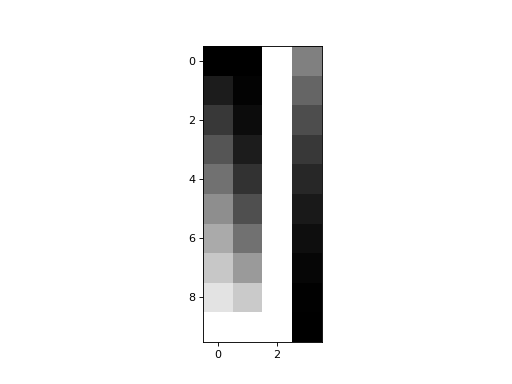
Now let’s add a fourth column that is a weighted sum of the first three:
>>> X_not_full_rank = np.zeros((10, 4))
>>> X_not_full_rank[:, :3] = X
>>> X_not_full_rank[:, 3] = np.dot(X, [-1, 0.5, 0.5])
>>> plt.imshow(X_not_full_rank)
<...>

matrix_rank is up to the job:
>>> npl.matrix_rank(X_not_full_rank)
3
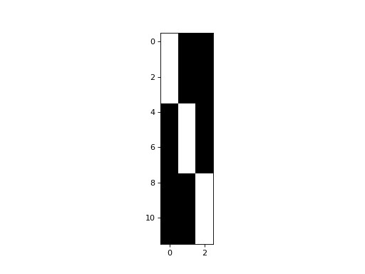
A more typical situation with design matrices, is that we have some dummy variable columns coding for group membership, that sum up to a column of ones.
>>> dummies = np.kron(np.eye(3), np.ones((4, 1)))
>>> plt.imshow(dummies)
<...>

So far, so good:
>>> npl.matrix_rank(dummies)
3
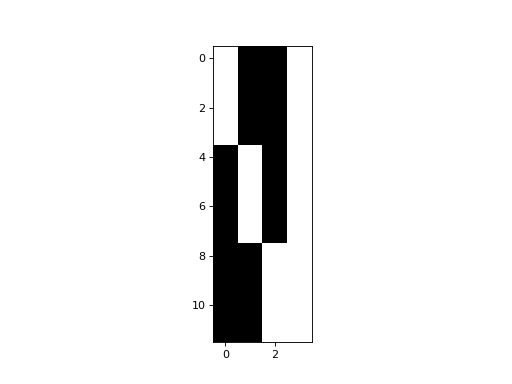
If we add a column of ones to model the mean, we now have an extra column that is a linear combination of other columns in the model:
>>> dummies_with_mean = np.hstack((dummies, np.ones((12, 1))))
>>> plt.imshow(dummies_with_mean)
<...>

>>> npl.matrix_rank(dummies_with_mean)
3
A matrix is full rank if the matrix rank is the same as the number of columns / rows. That is, a matrix is full rank if all the columns (or rows) are independent.
If a matrix is not full rank then it is rank deficient.