\(\newcommand{L}[1]{\| #1 \|}\newcommand{VL}[1]{\L{ \vec{#1} }}\newcommand{R}[1]{\operatorname{Re}\,(#1)}\newcommand{I}[1]{\operatorname{Im}\, (#1)}\)
Fourier without the ei
Introduction
The standard equations for discrete Fourier transforms (DFTs) involve exponentials to the power of \(i\) - the imaginary unit. I personally find these difficult to think about, and it turns out, the DFT is fairly easy to recast in terms of \(\sin\) and \(\cos\). This page goes through this process, and tries to show how thinking in this way can explain some features of the DFT.
How hard is the mathematics?
You will not need heavy mathematics to follow this page. If you don’t remember the following concepts you might want to brush up on them. There are also links to proofs and explanations for these ideas in the page as we go along:
basic trigonometry (SOH CAH TOA, Pythagoras’ theorem);
the angle sum rule;
You will not need to go deep into complex numbers, but see Refresher on complex numbers.
Loading and configuring code libraries
Load and configure the Python libraries we will use:
>>> import numpy as np  # the Python array package
>>> import matplotlib.pyplot as plt  # the Python plotting package
>>> # Tell numpy to print numbers to 4 decimal places only
>>> np.set_printoptions(precision=4, suppress=True)
Hint
If running in the IPython console, consider running %matplotlib to enable
interactive plots. If running in the Jupyter Notebook, use %matplotlib
inline.
Some actual numbers to start
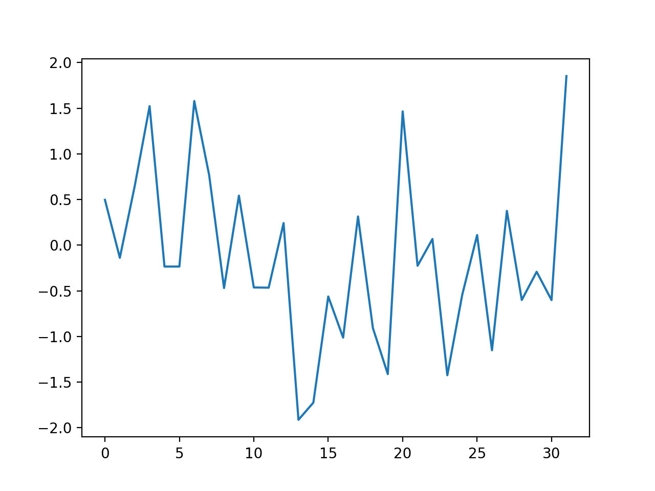
Let us start with a DFT of some data.
>>> # An example input vector
>>> x = np.array(
...     [ 0.4967, -0.1383,  0.6477,  1.523 , -0.2342, -0.2341,  1.5792,
...       0.7674, -0.4695,  0.5426, -0.4634, -0.4657,  0.242 , -1.9133,
...      -1.7249, -0.5623, -1.0128,  0.3142, -0.908 , -1.4123,  1.4656,
...      -0.2258,  0.0675, -1.4247, -0.5444,  0.1109, -1.151 ,  0.3757,
...      -0.6006, -0.2917, -0.6017,  1.8523])
>>> N = len(x)
>>> N
32
>>> plt.plot(x)
[...]

>>> # Now the DFT
>>> X = np.fft.fft(x)
>>> X
array([-4.3939+0.j    ,  9.0217-3.7036j, -0.5874-6.2268j,  2.5184+3.7749j,
        0.5008-0.8433j,  1.2904-0.4024j,  4.3391+0.8079j, -6.2614+2.1596j,
        1.8974+2.4889j,  0.1042+7.6169j,  0.3606+5.162j ,  4.7965+0.0755j,
       -5.3064-3.2329j,  4.6237+1.5287j, -2.1211+4.4873j, -4.0175-0.3712j,
       -2.0297+0.j    , -4.0175+0.3712j, -2.1211-4.4873j,  4.6237-1.5287j,
       -5.3064+3.2329j,  4.7965-0.0755j,  0.3606-5.162j ,  0.1042-7.6169j,
        1.8974-2.4889j, -6.2614-2.1596j,  4.3391-0.8079j,  1.2904+0.4024j,
        0.5008+0.8433j,  2.5184-3.7749j, -0.5874+6.2268j,  9.0217+3.7036j])
Notice that X - the output of the forward DFT - is a vector of complex
numbers.
Each value in X gives the scaling for a sinusoid for a particular
frequency.
If the input to the DFT is real, as here, then:
The real part of
Xhas the scaling for a cosine at the particular frequency;The imaginary part of
Xhas the scaling for a sine at that frequency.
There are some patterns to these numbers. Notice that the numbers at index 0
and N/2 (=16) have 0 for their imaginary part, and that X[17:] is a mirror
image of X[1:16], with the imaginary parts having the opposite sign.
>>> X[1:16]
array([ 9.0217-3.7036j, -0.5874-6.2268j,  2.5184+3.7749j,  0.5008-0.8433j,
        1.2904-0.4024j,  4.3391+0.8079j, -6.2614+2.1596j,  1.8974+2.4889j,
        0.1042+7.6169j,  0.3606+5.162j ,  4.7965+0.0755j, -5.3064-3.2329j,
        4.6237+1.5287j, -2.1211+4.4873j, -4.0175-0.3712j])
>>> X[17:][::-1]
array([ 9.0217+3.7036j, -0.5874+6.2268j,  2.5184-3.7749j,  0.5008+0.8433j,
        1.2904+0.4024j,  4.3391-0.8079j, -6.2614-2.1596j,  1.8974-2.4889j,
        0.1042-7.6169j,  0.3606-5.162j ,  4.7965-0.0755j, -5.3064+3.2329j,
        4.6237-1.5287j, -2.1211-4.4873j, -4.0175+0.3712j])
These features constitute conjugate symmetry and are always true of a DFT on real numbers. We will soon see why.
When we do the inverse DFT on X we return the original values of our
input x, but as complex numbers with imaginary part 0:
>>> # Apply the inverse DFT to the output of the forward DFT
>>> x_back = np.fft.ifft(X)
>>> x_back
array([ 0.4967-0.j, -0.1383-0.j,  0.6477-0.j,  1.5230-0.j, -0.2342-0.j,
       -0.2341+0.j,  1.5792+0.j,  0.7674+0.j, -0.4695-0.j,  0.5426-0.j,
       -0.4634-0.j, -0.4657+0.j,  0.2420-0.j, -1.9133-0.j, -1.7249-0.j,
       -0.5623+0.j, -1.0128-0.j,  0.3142+0.j, -0.9080+0.j, -1.4123+0.j,
        1.4656+0.j, -0.2258+0.j,  0.0675+0.j, -1.4247-0.j, -0.5444+0.j,
        0.1109+0.j, -1.1510+0.j,  0.3757-0.j, -0.6006-0.j, -0.2917-0.j,
       -0.6017-0.j,  1.8523-0.j])
Traditional notation for the discrete Fourier transform
Let us say we have a vector of \(N\) values in time, or space \(\vec{x} = [x_0, x_1 ... x_{N-1}]\). We generally index \(\vec{x}\) with subscript \(n\), so the sample at index \(n\) is \(x_n\).
The DFT converts \(\vec{x}\) from a vector in time, or space, to a vector \(\vec{X}\) representing temporal or spatial frequency components.
We will call our original \(\vec{x}\) the signal, meaning, the signal not transformed to frequency.
The DFT converts \(\vec{x}\) to \(\vec{X}\) where \(\vec{X} = [X_0, X_1, ... X_{N-1}]\). We generally index \(\vec{X}\) with subscript \(k\), so the sample at index \(k\) is \(X_k\).
Here is the equation for the discrete Fourier transform:
This is the transform from signal to frequency. We will call this the forward Fourier transform.
Here is the equation for the inverse Fourier transform:
The inverse Fourier transform converts from frequency back to signal.
DFT and FFT
The fast Fourier transform (FFT) refers to a particular set of - er - fast algorithms for calculating the DFT. It is common, but confusing, to use “FFT” to mean DFT.
Rewriting the DFT without the \(e^i\)
Why rewrite without \(e^i\)?
The forward and inverse equations are very similar; both share a term \(e^{iz}\), where \(z = -2 \pi \frac{k}{N} n\) for the forward transform; \(z = 2 \pi \frac{k}{N} n\) for the inverse transform.
Some people are used to looking at the form \(e^{iz}\) and thinking “aha, that’s a rotation around a circle”. Apparently this is an intuition that builds up over time working with these sorts of equations.
Unfortunately, some of us find it hard to think in complex exponentials, or in terms of complex numbers.
So, in this tutorial, we will express the Fourier transform in terms of \(\sin\) and \(\cos\). We will be using complex numbers, but almost entirely as a pair of numbers to represent two components of the same thing, rather than a single number with a real and imaginary part.
Having said that, we will need some very basic properties of complex and imaginary numbers - see Refresher on complex numbers.
How to rewrite without \(e^i\)
Our first tool in this enterprise is Euler’s formula:
This is the basis for thinking of \(e^{i \theta}\) as being rotation around a circle, of which you will hear no more in this page. In our case, it allows us to rewrite the forward and inverse Fourier transforms:
First let’s define a new value \(D\), that depends on \(N\) - the number of observations in our vector \(\vec{x}\).
With that value:
We can simplify this further, because, for any angle \(\alpha\):
Following the same logic for the inverse transform:
Rewriting the DFT with vectors
We can write the elements inside the DFT summations as values from vectors:
where:
Call \(\vec{r^k}\) the angle vector for \(k\). This vector depend only on \(k\) and \(N\).
Substituting the value of \(D\) (equation (3)):
Now define:
We have:
Given the definition of the Vector dot product, we can write the forward DFT as:
Frequency as cycles across the sample vector
The key to the frequencies in the DFT is in the \(n k D = k 2 \pi \frac{n}{N}\) values that we have put into the angle vector \(\vec{r^k}\).
The \(k\) in \(\vec{r^k}\) gives the number of cycles across all \(N\) values of \(\vec{x}\).
For example, consider the case of \(k = 1\):
Here are the values in Python:
>>> vec_n = np.arange(N)
>>> vec_r_1 = 2 * np.pi * vec_n / float(N)
>>> vec_r_1
array([ 0.    ,  0.1963,  0.3927,  0.589 ,  0.7854,  0.9817,  1.1781,
        1.3744,  1.5708,  1.7671,  1.9635,  2.1598,  2.3562,  2.5525,
        2.7489,  2.9452,  3.1416,  3.3379,  3.5343,  3.7306,  3.927 ,
        4.1233,  4.3197,  4.516 ,  4.7124,  4.9087,  5.1051,  5.3014,
        5.4978,  5.6941,  5.8905,  6.0868])
The values \(\frac{0}{N}, \frac{1}{N}, \ldots \frac{N-1}{N}\) are fractions of the number of samples \(N\), running from 0 to close to 1. Now multiplied by \(2 \pi\), the values run from 0 to close to \(2 \pi\) and therefore give angles around a circle.
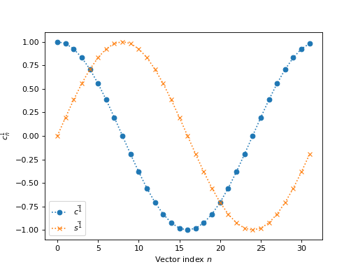
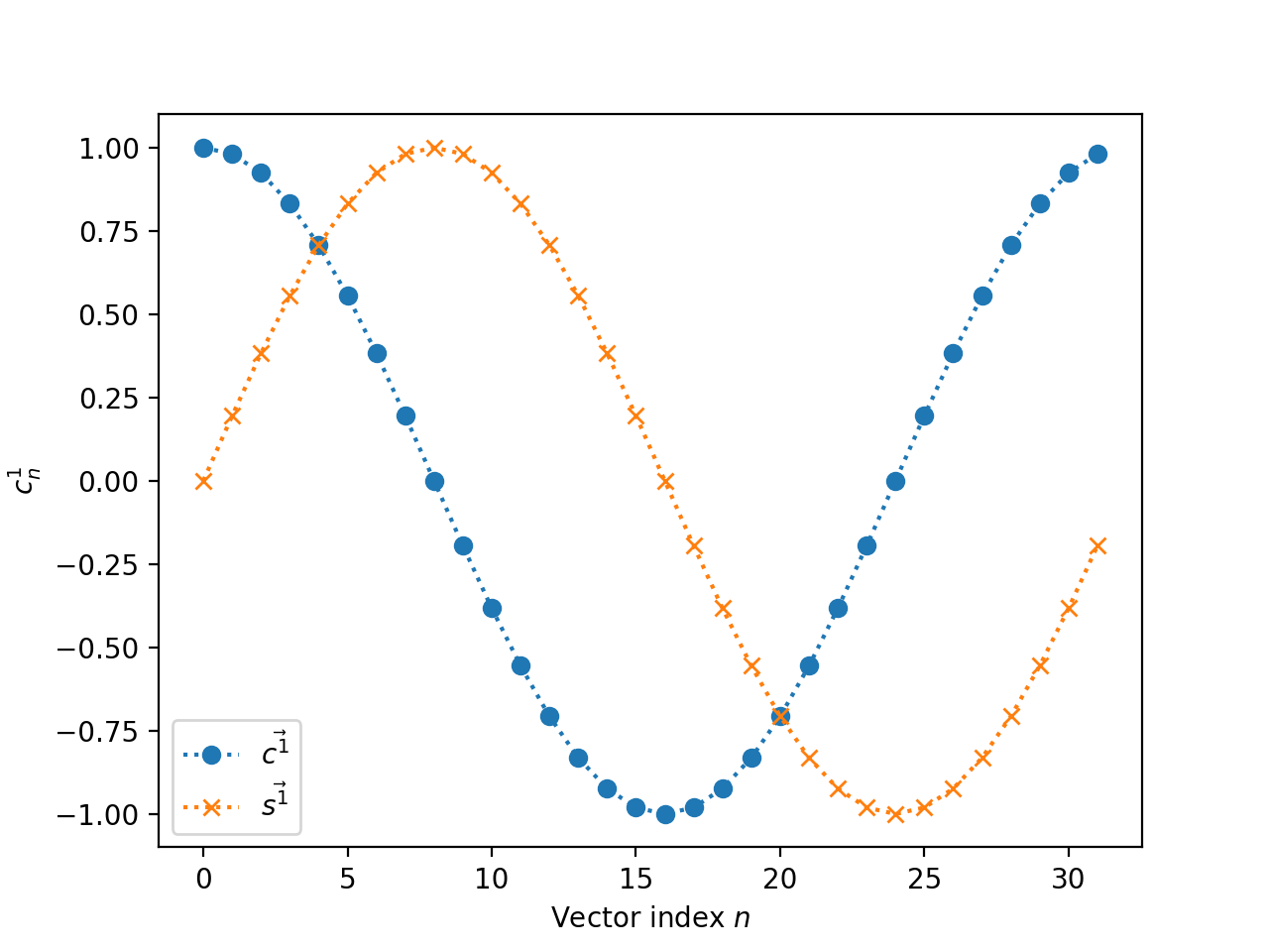
The vector \(\vec{r^1}\) gives \(\vec{c^1}, \vec{s^1}\) with a single cycle:
>>> vec_c_1 = np.cos(vec_r_1)
>>> vec_s_1 = np.sin(vec_r_1)
>>> plt.plot(vec_n, vec_c_1, 'o:', label=r'$\vec{c^1}$')
[...]
>>> plt.plot(vec_n, vec_s_1, 'x:', label=r'$\vec{s^1}$')
[...]
>>> plt.xlabel('Vector index $n$')
<...>
>>> plt.ylabel('$c^1_n$')
<...>
>>> plt.legend()
<...>

\(k = 2\) gives 2 cycles across the N values:
>>> vec_r_2 = vec_r_1 * 2
>>> vec_c_2 = np.cos(vec_r_2)
>>> vec_s_2 = np.sin(vec_r_2)
>>> plt.plot(vec_n, vec_c_2, 'o:', label=r'$\vec{c^2}$')
[...]
>>> plt.plot(vec_n, vec_s_2, 'x:', label=r'$\vec{s^2}$')
[...]
>>> plt.xlabel('Vector index $n$')
<...>
>>> plt.ylabel('$c^2_n$')
<...>
>>> plt.legend()
<...>

Calculating the DFT with vectors
First DFT output value is the vector sum
Consider \(\vec{r^0}, \vec{c^0}, \vec{s^0}\):
Therefore:
The first value in the DFT output vector is the sum of the values in \(\vec{x}\). If \(\vec{x}\) has real and not complex values, as here, then \(X_0\) has zero imaginary part:
>>> print(np.sum(x))
-4.3939
>>> print(X[0])
(-4.3939+0j)
Now let’s imagine that our input vector is a constant, say a vector of ones. What is the DFT?
>>> vec_ones = np.ones(N)
>>> np.fft.fft(vec_ones)
array([ 32.+0.j,   0.+0.j,   0.+0.j,   0.+0.j,   0.+0.j,   0.+0.j,
         0.+0.j,   0.+0.j,   0.+0.j,   0.+0.j,   0.+0.j,   0.+0.j,
         0.+0.j,   0.+0.j,   0.+0.j,   0.+0.j,   0.+0.j,   0.+0.j,
         0.+0.j,   0.+0.j,   0.+0.j,   0.+0.j,   0.+0.j,   0.+0.j,
         0.+0.j,   0.+0.j,   0.+0.j,   0.+0.j,   0.+0.j,   0.+0.j,
         0.+0.j,   0.+0.j])
We were expecting the first value of 32, because it is the sum of 32 values of one. All the other values are 0. This is because all of \(\vec{c^1}, \vec{c^2}, \ldots, \vec{c^{N-1}}\) and all of \(\vec{s^1}, \vec{s^2}, \ldots, \vec{s^{N-1}}\) sum to zero, and therefore the dot product of all these vectors with a constant vector is also zero.
Second DFT output corresponds to a sinusoid at frequency \(1 / N\).
We have already seen \(\vec{r^1}, \vec{c^1}, \vec{s^1}\).
\(\vec{c^1}, \vec{s^1}\) are the cosine, sine at frequency 1 / N where one unit is the distance between two consecutive samples in \(\vec{x}\).
>>> print(x.dot(vec_c_1), x.dot(vec_s_1))
9.02170725475 3.70356074953
>>> print(X[1])
(9.02170725475-3.70356074953j)
This confirms our calculation gives the same result as numpy’s DFT, but isn’t very revealing.
Let’s make another input vector \(\vec{v}\) that is a cosine at the same frequency as \(\vec{c^1}\). Start with \(\vec{v} = \vec{c^1}\).
Our prediction for the DFT of \(\vec{v}\) is:
In fact, as you can see in The Fourier basis, it is a property of the \(\vec{c^k}, \vec{s^k}\) vectors that, for all \(k, N\):
Remember from Vector length that, for any vector \(\vec{w}\), we can write \(\vec{w} \cdot \vec{w}\) as \(\VL{w}^2\)
So:
The Fourier basis also shows that \(\VL{c_1}^2 = N / 2\) for all N. More generally \(\VL{c_p}^2 = \VL{s_p}^2 = N / 2\) for all \(p \notin {0, N/2}\).
So:
>>> vec_v = vec_c_1
>>> V = np.fft.fft(vec_v)
>>> V
array([ -0.+0.j,  16.-0.j,   0.+0.j,   0.+0.j,  -0.-0.j,   0.+0.j,
         0.+0.j,   0.+0.j,   0.-0.j,   0.+0.j,  -0.+0.j,   0.+0.j,
         0.+0.j,  -0.+0.j,   0.-0.j,   0.+0.j,   0.+0.j,   0.+0.j,
         0.+0.j,  -0.+0.j,   0.-0.j,  -0.+0.j,  -0.-0.j,  -0.+0.j,
         0.+0.j,  -0.+0.j,   0.-0.j,  -0.+0.j,  -0.+0.j,  -0.+0.j,
         0.-0.j,  16.-0.j])
Notice that \(V_{N-1} = N/2 = V_1\). This is the property of conjugate symmetry. It is so because of the properties of the vectors \(\vec{c^k}\). As you see in The Fourier basis \(\vec{c_1} = \vec{c_{N-1}}\), and, more generally \(\vec{c_p} = \vec{c_{N-p}}\) for \(p \in 1, 2 \ldots, N / 2\).
Adding a scaling factor to the cosine
Now set \(\vec{v} = a \vec{c^1}\) where \(a\) is a constant:
By the properties of the dot product:
>>> a = 3
>>> vec_v = a * vec_c_1
>>> np.fft.fft(vec_v)
array([ -0.+0.j,  48.-0.j,   0.+0.j,   0.+0.j,  -0.-0.j,   0.+0.j,
         0.+0.j,   0.+0.j,   0.-0.j,   0.+0.j,  -0.-0.j,   0.+0.j,
        -0.+0.j,  -0.+0.j,   0.-0.j,   0.+0.j,   0.+0.j,   0.+0.j,
         0.+0.j,  -0.+0.j,  -0.-0.j,  -0.+0.j,  -0.+0.j,  -0.+0.j,
         0.+0.j,  -0.+0.j,   0.-0.j,  -0.+0.j,  -0.+0.j,  -0.+0.j,
         0.-0.j,  48.-0.j])
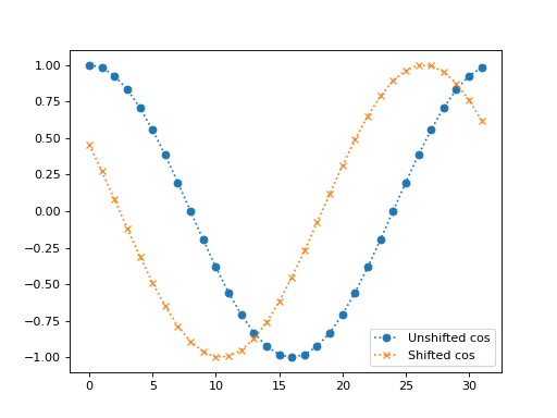
Adding a phase shift brings the sine into play
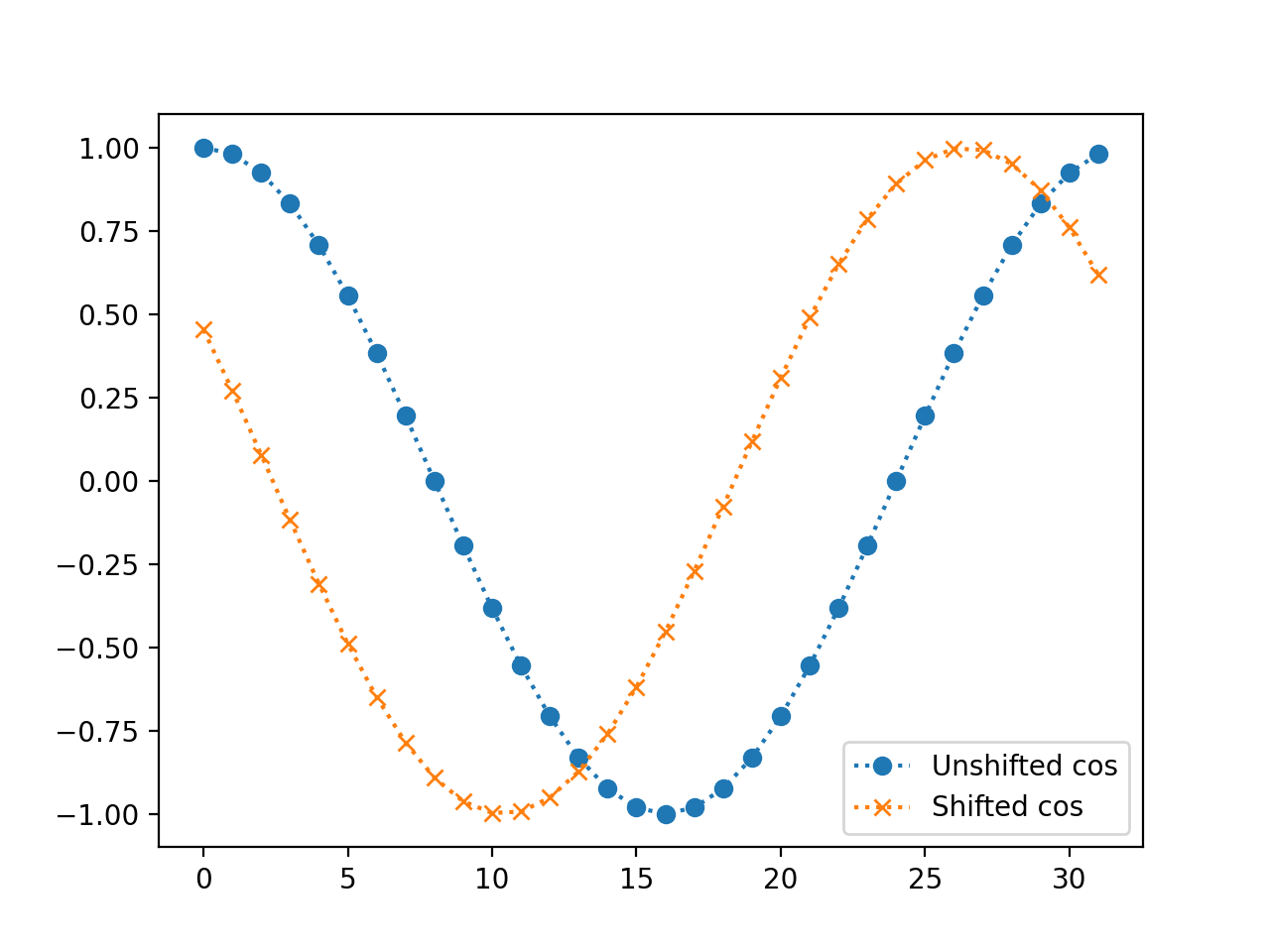
What happens if we add a phase shift of \(\beta\) radians to the input cosine?
>>> beta = 1.1
>>> vec_v = np.cos(vec_r_1 + beta)
>>> plt.plot(vec_n, vec_c_1, 'o:', label='Unshifted cos')
[...]
>>> plt.plot(vec_n, vec_v, 'x:', label='Shifted cos')
[...]
>>> plt.legend()
<...>
We can rewrite the shifted cosine using the The angle sum rule:
So:
Now apply the vector dot products to get \(V_1\):
Do we get this answer from the DFT?
>>> print(np.cos(beta) * (N / 2.), np.sin(beta) * (N / 2.))
7.25753794281 14.259317761
>>> np.fft.fft(vec_v)
array([-0.0000 +0.j    ,  7.2575+14.2593j,  0.0000 +0.j    ,
        0.0000 +0.j    ,  0.0000 +0.j    ,  0.0000 +0.j    ,
       -0.0000 +0.j    ,  0.0000 -0.j    , -0.0000 -0.j    ,
       -0.0000 +0.j    , -0.0000 -0.j    ,  0.0000 +0.j    ,
       -0.0000 +0.j    ,  0.0000 -0.j    ,  0.0000 +0.j    ,
        0.0000 +0.j    , -0.0000 +0.j    ,  0.0000 +0.j    ,
        0.0000 -0.j    ,  0.0000 +0.j    , -0.0000 -0.j    ,
        0.0000 +0.j    , -0.0000 +0.j    ,  0.0000 +0.j    ,
       -0.0000 +0.j    , -0.0000 +0.j    , -0.0000 -0.j    ,
       -0.0000 +0.j    ,  0.0000 -0.j    , -0.0000 +0.j    ,
        0.0000 -0.j    ,  7.2575-14.2593j])
Notice that \(V_{N-1}\) has the same value as \(V_{1}\), but with the imaginary part flipped in sign. This is the conjugate in conjugate symmetry. It comes about because of the construction of the vectors \(\vec{s^k}\). As you see in The Fourier basis \(\vec{s_1} = -\vec{s_{N-1}}\), and, more generally \(\vec{s_p} = -\vec{s_{N-p}}\) for \(p \in 1, 2 \ldots, N / 2\).
Reconstructing amplitude and phase from the DFT
To complete our journey into \(X_1\), let us add a scaling \(a\) to the phase-shifted cosine:
This gives us:
>>> print(a * np.cos(beta) * (N / 2.), a * np.sin(beta) * (N / 2.))
21.7726138284 42.7779532829
>>> vec_v = a * np.cos(vec_r_1 + beta)
>>> np.fft.fft(vec_v)
array([ -0.0000 +0.j   ,  21.7726+42.778j,   0.0000 +0.j   ,
         0.0000 +0.j   ,   0.0000 +0.j   ,   0.0000 +0.j   ,
        -0.0000 +0.j   ,   0.0000 -0.j   ,  -0.0000 -0.j   ,
        -0.0000 +0.j   ,  -0.0000 -0.j   ,   0.0000 +0.j   ,
        -0.0000 +0.j   ,   0.0000 -0.j   ,   0.0000 +0.j   ,
         0.0000 +0.j   ,  -0.0000 +0.j   ,   0.0000 +0.j   ,
         0.0000 -0.j   ,   0.0000 +0.j   ,  -0.0000 -0.j   ,
         0.0000 +0.j   ,  -0.0000 +0.j   ,   0.0000 +0.j   ,
        -0.0000 +0.j   ,  -0.0000 +0.j   ,  -0.0000 -0.j   ,
        -0.0000 +0.j   ,   0.0000 -0.j   ,  -0.0000 +0.j   ,
         0.0000 -0.j   ,  21.7726-42.778j])
What if I want to reconstruct \(a\) and \(\beta\) from the DFT coefficients?
From (4):
So:
By Pythagoras:
>>> X_1 = np.fft.fft(vec_v)[1]
>>> np.sqrt(np.real(X_1)**2 + np.imag(X_1)**2)
47.999999999999993
>>> 3 * N / 2.
48.0
We can get the angle \(\beta\) in a similar way:
np.arccos is the inverse of np.cos:
>>> np.real(X_1) / (a * N / 2.)
0.4535961214255782
>>> np.cos(beta)
0.45359612142557731
>>> np.arccos(np.real(X_1) / (a * N / 2.))
1.099999999999999
In fact, these are the calculations done by the standard np.abs, np.angle
functions:
>>> np.abs(X_1)
47.999999999999993
>>> np.angle(X_1)
1.099999999999999