$$

Convolution

Neural and hemodynamic models

In functional MRI (FMRI), we often have the subjects do a task in the scanner. For example, we might have the subject lying looking at a fixation cross on the screen for most of the time, and sometimes show a very brief burst of visual stimulation, such as a flashing checkerboard.

We will call each burst of stimulation an event.

The FMRI signal comes about first through changes in neuronal firing, and then by blood flow responses to the changes in neuronal firing. In order to predict the FMRI signal to an event, we first need a prediction (model) of the changes in neuronal firing, and second we need a prediction (model) of how the blood flow will change in response to the neuronal firing.

So we have a two-stage problem:

• predict the neuronal firing to the event (make a neuronal firing model);

• predict the blood flow changes caused by the neuronal firing (a hemodynamic model).

Convolution is a simple way to create a hemodynamic model from a neuronal firing model.

The neuronal firing model

The neuronal firing model is our prediction of the profile of neural activity in response to the event.

For example, in this case, with a single stimulation, we might predict that, as soon as the visual stimulation went on, the cells in the visual cortex instantly increased their firing, and kept firing at the same rate while the stimulation was on.

In that case, our neural model of an event starting at 4 seconds, lasting 5 seconds, might look like this:

>>> import numpy as np
>>> import matplotlib.pyplot as plt

Hint

If running in the IPython console, consider running %matplotlib to enable interactive plots. If running in the Jupyter Notebook, use %matplotlib inline.

>>> times = np.arange(0, 40, 0.1)
>>> n_time_points = len(times)
>>> neural_signal = np.zeros(n_time_points)
>>> neural_signal[(times >= 4) & (times < 9)] = 1
>>> plt.plot(times, neural_signal)
[...]
>>> plt.xlabel('time (seconds)')
<...>
>>> plt.ylabel('neural signal')
<...>
>>> plt.ylim(0, 1.2)
(...)
>>> plt.title("Neural model for 5 second event starting at time 4")
<...>

(png, hires.png, pdf)

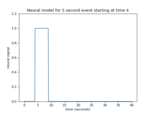
This type of simple off - on - off model is a boxcar function.

Of course we could have had another neural model, with the activity gradually increasing, or starting high and then dropping, but let us stick to this simple model for now.

Now we need to predict our hemodynamic signal, given our prediction of neuronal firing.

The impulse response

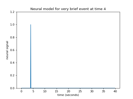
Let’s simplify a little by specifying that the event was really short. Call this event — an impulse. This simplifies our neural model to a single spike in time instead of the sustained rise of the box-car function.

>>> neural_signal = np.zeros(n_time_points)
>>> i_time_4 = np.where(times == 4)[0][0]  # index of value 4 in "times"
>>> neural_signal[i_time_4] = 1  # A single spike at time == 4
>>> plt.plot(times, neural_signal)
[...]
>>> plt.xlabel('time (seconds)')
<...>
>>> plt.ylabel('neural signal')
<...>
>>> plt.ylim(0, 1.2)
(...)
>>> plt.title("Neural model for very brief event at time 4")
<...>

(png, hires.png, pdf)

Let us now imagine that I know what the hemodynamic response will be to such an impulse. I might have got this estimate from taking the FMRI signal following very brief events, and averaging over many events. Here is one such estimate of the hemodynamic response to a very brief stimulus:

>>> def hrf(t):
...     "A hemodynamic response function"
...     return t ** 8.6 * np.exp(-t / 0.547)

>>> hrf_times = np.arange(0, 20, 0.1)
>>> hrf_signal = hrf(hrf_times)
>>> plt.plot(hrf_times, hrf_signal)
[...]
>>> plt.xlabel('time (seconds)')
<...>
>>> plt.ylabel('BOLD signal')
<...>
>>> plt.title('Estimated BOLD signal for event at time 0')
<...>

(png, hires.png, pdf)

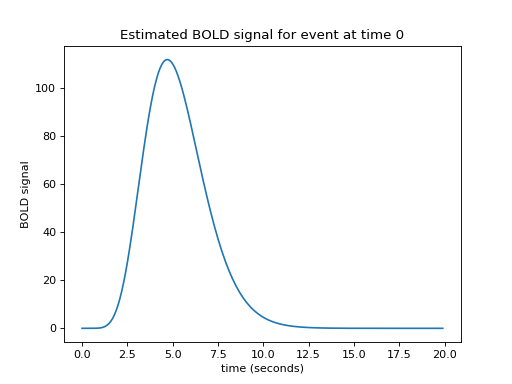
This is the hemodynamic response to a neural impulse. In signal processing terms this is the hemodynamic impulse response function. It is usually called the hemodynamic response function (HRF), because it is a function that gives the predicted hemodynamic response at any given time following an impulse at time 0.

Building the hemodynamic output from the neural input

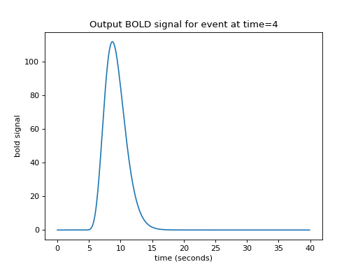
We now have an easy way to predict the hemodynamic output from our single impulse at time 4. We take the HRF (prediction for an impulse starting at time 0), and shift it by 4 seconds-worth to give our predicted output:

>>> n_hrf_points = len(hrf_signal)
>>> bold_signal = np.zeros(n_time_points)
>>> bold_signal[i_time_4:i_time_4 + n_hrf_points] = hrf_signal
>>> plt.plot(times, bold_signal)
[...]
>>> plt.xlabel('time (seconds)')
<...>
>>> plt.ylabel('bold signal')
<...>
>>> plt.title('Output BOLD signal for event at time=4')
<...>

(png, hires.png, pdf)

Our impulse so far has an amplitude of 1. What if the impulse was twice as strong, with an amplitude of 2?

>>> neural_signal[i_time_4] = 2  # An impulse with amplitude 2
>>> plt.plot(times, neural_signal)
[...]
>>> plt.xlabel('time (seconds)')
<...>
>>> plt.ylabel('neural signal')
<...>
>>> plt.ylim(0, 2.2)
(...)
>>> plt.title('Neural model for amplitude 2 impulse')
<...>

(png, hires.png, pdf)

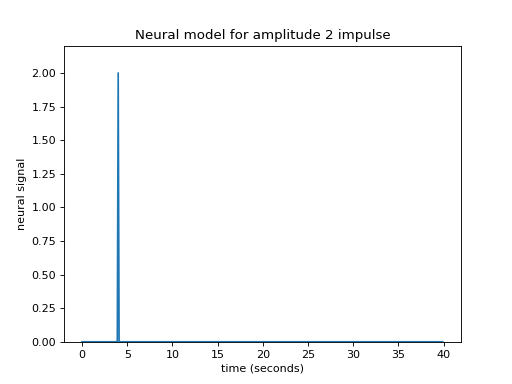
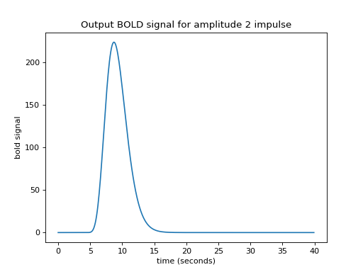
Maybe I can make the assumption that, if the impulse is twice as large then the response will be twice as large. This is the assumption that the response scales linearly with the impulse.

Now I can predict the output for an impulse of amplitude 2 by taking my HRF, shifting by 4, as before, and then multiplying the HRF by 2:

>>> bold_signal = np.zeros(n_time_points)
>>> bold_signal[i_time_4:i_time_4 + n_hrf_points] = hrf_signal * 2
>>> plt.plot(times, bold_signal)
[...]
>>> plt.xlabel('time (seconds)')
<...>
>>> plt.ylabel('bold signal')
<...>
>>> plt.title('Output BOLD signal for amplitude 2 impulse')
<...>

(png, hires.png, pdf)

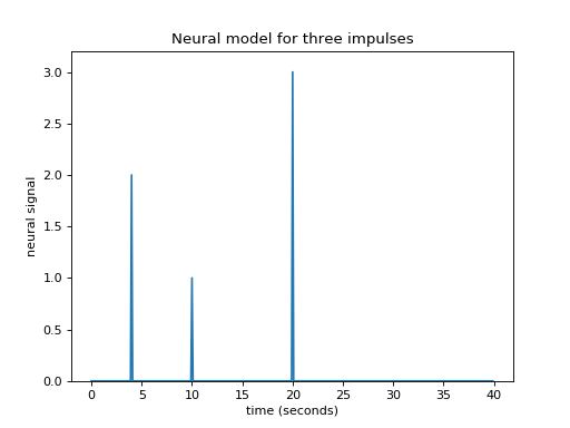
What if I have several impulses? For example, imagine I had an impulse amplitude 2 at time == 4, then another of amplitude 1 at time == 10, and another of amplitude 3 at time == 20.

>>> neural_signal[i_time_4] = 2  # An impulse with amplitude 2
>>> i_time_10 = np.where(times == 10)[0][0]  # index of value 10 in "times"
>>> neural_signal[i_time_10] = 1  # An impulse with amplitude 1
>>> i_time_20 = np.where(times == 20)[0][0]  # index of value 20 in "times"
>>> neural_signal[i_time_20] = 3  # An impulse with amplitude 3
>>> plt.plot(times, neural_signal)
[...]
>>> plt.xlabel('time (seconds)')
<...>
>>> plt.ylabel('neural signal')
<...>
>>> plt.ylim(0, 3.2)
(...)
>>> plt.title('Neural model for three impulses')
<...>

(png, hires.png, pdf)

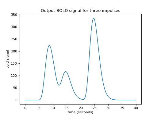
Maybe I can also make the assumption that the response to an impulse will be exactly the same over time. The response to any given impulse at time 10 will be the same as the response to the same impulse at time 4 or at time 30.

In that case my job is still simple. For the impulse amplitude 2 at time == 4, I add the HRF shifted to start at time == 4, and scaled by 2. To that result I then add the HRF shifted to time == 10 and scaled by 1. Finally, I further add the HRF shifted to time == 20 and scaled by 3:

>>> bold_signal = np.zeros(n_time_points)
>>> bold_signal[i_time_4:i_time_4 + n_hrf_points] = hrf_signal * 2
>>> bold_signal[i_time_10:i_time_10 + n_hrf_points] += hrf_signal * 1
>>> bold_signal[i_time_20:i_time_20 + n_hrf_points] += hrf_signal * 3
>>> plt.plot(times, bold_signal)
[...]
>>> plt.xlabel('time (seconds)')
<...>
>>> plt.ylabel('bold signal')
<...>
>>> plt.title('Output BOLD signal for three impulses')
<...>

(png, hires.png, pdf)

At the moment, an impulse is an event that lasts for just one time point. In our case, the time vector (times in the code above) has one point for every 0.1 seconds (10 time points per second).

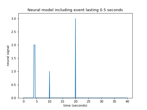
What happens if an event lasts for 0.5 seconds? Maybe I can assume that an event lasting 0.5 seconds has exactly the same effect as 5 impulses 0.1 seconds apart:

>>> neural_signal[i_time_4:i_time_4 + 5] = 2
>>> plt.plot(times, neural_signal)
[...]
>>> plt.xlabel('time (seconds)')
<...>
>>> plt.ylabel('neural signal')
<...>
>>> plt.ylim(0, 3.2)
(...)
>>> plt.title('Neural model including event lasting 0.5 seconds')
<...>

(png, hires.png, pdf)

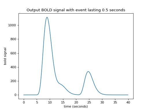
Now I need to add a new shifted HRF for the impulse corresponding to time == 4, and for time == 4.1 and so on until time == 4.4:

>>> bold_signal = np.zeros(n_time_points)
>>> for i in range(5):
...     bold_signal[i_time_4 + i:i_time_4  + i + n_hrf_points] += hrf_signal * 2
>>> bold_signal[i_time_10:i_time_10 + n_hrf_points] += hrf_signal * 1
>>> bold_signal[i_time_20:i_time_20 + n_hrf_points] += hrf_signal * 3
>>> plt.plot(times, bold_signal)
[...]
>>> plt.xlabel('time (seconds)')
<...>
>>> plt.ylabel('bold signal')
<...>
>>> plt.title('Output BOLD signal with event lasting 0.5 seconds')
<...>

(png, hires.png, pdf)

Working out an algorithm

Now we have a general algorithm for making our output hemodynamic signal from our input neural signal:

1. Start with an output vector that is a vector of zeros;

2. For each index $i$ in the input vector (the neural signal):

   3. Prepare a shifted copy of the HRF vector, starting at $i$. Call this the shifted HRF vector;

   4. Multiply the shifted HRF vector by the value in the input at index $i$, to give the shifted, scaled HRF vector;

   5. Add the shifted scaled HRF vector to the output.

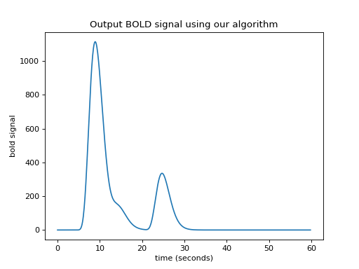
There is a little problem with our algorithm — the length of the output vector.

Imagine that our input (neural) vector is N time points long. Say the original HRF vector is M time points long.

In our algorithm, when the iteration gets to the last index of the input vector ($i=N-1$), the shifted scaled HRF vector will, as ever, be M points long. If the output vector is the same length as the input vector, we can add only the first point of the new scaled HRF vector to the last point of the output vector, but all the subsequent values of the scaled HRF vector extend off the end of the output vector and have no corresponding index in the output. The way to solve this is to extend the output vector by the necessary M-1 points. Now we can do our algorithm in code.

>>> N = n_time_points
>>> M = n_hrf_points
>>> bold_signal = np.zeros(N + M - 1)  # adding the tail
>>> for i in range(N):
...     input_value = neural_signal[i]
...     # Adding the shifted, scaled HRF
...     bold_signal[i : i + n_hrf_points] += hrf_signal * input_value
>>> # We have to extend 'times' to deal with more points in 'bold_signal'
>>> extra_times = np.arange(n_hrf_points - 1) * 0.1 + 40
>>> times_and_tail = np.concatenate((times, extra_times))
>>> plt.plot(times_and_tail, bold_signal)
[...]
>>> plt.xlabel('time (seconds)')
<...>
>>> plt.ylabel('bold signal')
<...>
>>> plt.title('Output BOLD signal using our algorithm')
<...>

(png, hires.png, pdf)

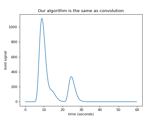
We have convolution

We now have — convolution. Here’s the same thing using the numpy convolve function:

>>> bold_signal = np.convolve(neural_signal, hrf_signal)
>>> plt.plot(times_and_tail, bold_signal)
[...]
>>> plt.xlabel('time (seconds)')
<...>
>>> plt.ylabel('bold signal')
<...>
>>> plt.title('Our algorithm is the same as convolution')
<...>

(png, hires.png, pdf)

Convolution with matrices

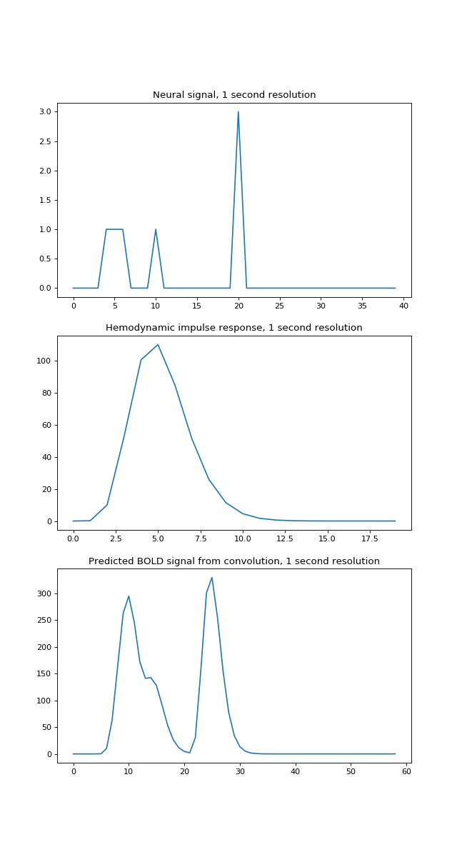
For what follows, it is a bit easier to see what is going on with a lower time resolution — say one time point per second. This time we’ll make the first event last 3 seconds:

>>> times = np.arange(0, 40)  # One time point per second
>>> n_time_points = len(times)
>>> neural_signal = np.zeros(n_time_points)
>>> neural_signal[4:7] = 1  # A 3 second event
>>> neural_signal[10] = 1
>>> neural_signal[20] = 3
>>> hrf_times = np.arange(20)
>>> hrf_signal = hrf(hrf_times)  # The HRF at one second time resolution
>>> n_hrf_points = len(hrf_signal)
>>> bold_signal = np.convolve(neural_signal, hrf_signal)
>>> times_and_tail = np.arange(n_time_points + n_hrf_points - 1)
>>> fig, axes = plt.subplots(3, 1, figsize=(8, 15))
>>> axes[0].plot(times, neural_signal)
[...]
>>> axes[0].set_title('Neural signal, 1 second resolution')
<...>
>>> axes[1].plot(hrf_times, hrf_signal)
[...]
>>> axes[1].set_title('Hemodynamic impulse response, 1 second resolution')
<...>
>>> axes[2].plot(times_and_tail, bold_signal)
[...]
>>> axes[2].set_title('Predicted BOLD signal from convolution, 1 second resolution')
<...>

(png, hires.png, pdf)

Our algorithm, which turned out to give convolution, had us add a shifted, scaled version of the HRF to the output, for every index. This is step 5 of our algorithm.

Now let us go back to our convolution algorithm. Imagine that, instead of adding the shifted scaled HRF to the output vector, we store each shifted scaled HRF as a row in an array, that has one row for each index in the input vector. Then we can get the same output vector as before by taking the sum across the columns of this array:

>>> N = n_time_points
>>> M = n_hrf_points
>>> shifted_scaled_hrfs = np.zeros((N, N + M - 1))
>>> for i in range(N):
...     input_value = neural_signal[i]
...     # Storing the shifted, scaled HRF
...     shifted_scaled_hrfs[i, i : i + n_hrf_points] = hrf_signal * input_value
>>> bold_signal_again = np.sum(shifted_scaled_hrfs, axis=0)

>>> # We check that the result is almost exactly the same
>>> # (allowing for tiny differences due to the order of +, * operations)
>>> import numpy.testing as npt
>>> npt.assert_almost_equal(bold_signal, bold_signal_again)

We can also do exactly the same operation by first making an array with the shifted HRFs, without scaling, and then multiplying each row by the corresponding input value, before doing the sum. Here we are doing the shifting first, and then the scaling, and then the sum. It all adds up to the same operation:

>>> # First we make the shifted HRFs
>>> shifted_hrfs = np.zeros((N, N + M - 1))
>>> for i in range(N):
...     # Storing the shifted HRF without scaling
...     shifted_hrfs[i, i : i + n_hrf_points] = hrf_signal
>>> # Then do the scaling
>>> shifted_scaled_hrfs = np.zeros((N, N + M - 1))
>>> for i in range(N):
...     input_value = neural_signal[i]
...     # Scaling the stored HRF by the input value
...     shifted_scaled_hrfs[i, :] = shifted_hrfs[i, :] * input_value
>>> # Then the sum
>>> bold_signal_again = np.sum(shifted_scaled_hrfs, axis=0)
>>> # This gives the same result, once again
>>> npt.assert_almost_equal(bold_signal, bold_signal_again)

The shifted_hrfs array looks like this as an image:

>>> plt.imshow(shifted_hrfs, cmap='gray', interpolation='nearest')
<...>

(png, hires.png, pdf)

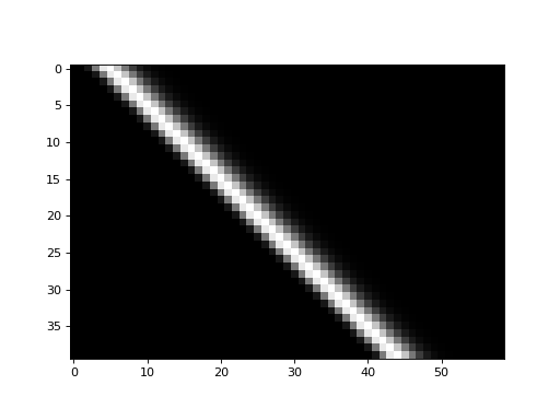
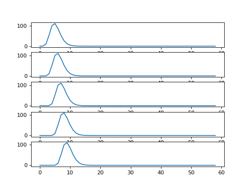
Each new row of shifted_hrfs corresponds to the HRF, shifted by one more column to the right:

>>> fig, axes = plt.subplots(5, 1)
>>> for row_no in range(5):
...     axes[row_no].plot(shifted_hrfs[row_no, :])
[...]

(png, hires.png, pdf)

Now remember matrix multiplication:

$$\begin{array}{r}\left(\begin{array}{c}xa+yb+zc\\ xd+ye+zf\end{array}\right)=\left(\begin{array}{ccc}x& y& z\end{array}\right)\left(\begin{array}{cc}a& d\\ b& e\\ c& f\end{array}\right)\end{array}$$

Now let us make our input neural vector into a 1 by N row vector. If we matrix multiply this vector onto the shifted_hrfs array (matrix), then we do the scaling of the HRFs and the sum operation, all in one go. Like this:

>>> def as_row_vector(v):
...     " Convert 1D vector to row vector "
...     return v.reshape((1, -1))

>>> neural_vector = as_row_vector(neural_signal)
>>> # The scaling and summing by the magic of matrix multiplication
>>> bold_signal_again = neural_vector.dot(shifted_hrfs)
>>> # This gives the same result as previously, yet one more time
>>> npt.assert_almost_equal(as_row_vector(bold_signal), bold_signal_again)

The matrix transpose rule says $(AB{)}^T=B^T{A}^T$ where $A^T$ is the transpose of matrix $A$. So we could also do this exact same operation by doing a matrix multiply of the transpose of shifted_hrfs onto the neural_signal as a column vector:

>>> bold_signal_again = shifted_hrfs.T.dot(neural_vector.T)
>>> # Exactly the same, but transposed
>>> npt.assert_almost_equal(as_row_vector(bold_signal), bold_signal_again.T)

In this last formulation, the shifted_hrfs matrix is the convolution matrix, in that (as we have just shown) you can apply the convolution of the HRF by matrix multiplying onto an input vector.

Convolution is like cross-correlation with the reversed HRF

We are now ready to show something slightly odd that arises from the way that convolution works.

Consider index $i$ in the input (neural) vector. Let’s say $i=25$. We want to get value index $i$ in the output (hemodynamic vector). What do we need to do?

Looking at our non-transposed matrix formulation, we see that value $i$ in the output is the matrix multiplication of the neural signal (row vector) by column $i$ in shifted_hrfs. Here is a plot of column 25 in shifted_hrfs:

>>> plt.plot(shifted_hrfs[:, 25])
[...]

(png, hires.png, pdf)

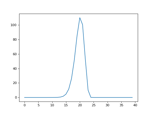
The column contains a reversed copy of the HRF signal, where the first value from the original HRF signal is at index 25 ($i$), the second value is at index 24 ($i-1$) and so on back to index 25 - 20 = 5. The reversed HRF follows from the way we constructed the rows of the original matrix. Each new HRF row was shifted across by one column, therefore, reading up the columns from the diagonals, will also give you the HRF shape.

Let us rephrase the matrix multiplication that gives us the value at index $i$ in the output vector. Call the neural input vector $\mathbf{n}$ with values $n_0,n_1...n_{N-1}$. Call the shifted_hrfs array $\mathbf{S}$ with $N$ rows and $N+M-1$ columns. ${\mathbf{S}}_{:,i}$ is column $i$ in $\mathbf{S}$.

So, the output value $o_i$ is given by the matrix multiplication of row $\mathbf{n}$ onto column ${\mathbf{S}}_{:,i}$. The matrix multiplication (dot product) gives us the usual sum of products as the output:

$$o_i=\sum _{j=0}^{N-1}{n}_j{S}_{j,i}$$

The formula above describes what is happening in the matrix multiplication in this piece of code:

>>> i = 25
>>> bold_i = neural_vector.dot(shifted_hrfs[:, i])

>>> npt.assert_almost_equal(bold_i, bold_signal[i])

Can we simplify the formula without using the shifted_hrfs $\mathbf{S}$ matrix? We saw above that column $i$ in shifted_hrfs contains a reversed HRF, starting at index $i$ and going backwards towards index 0.

The 1-second resolution HRF is our array hrf_signal. So shifted_hrfs[i, i] contains hrf_signal[0], shifted_hrfs[i-1, i] contains hrf_signal[1] and so on. In general, for any index $j$ into shifted_hrfs[:, i], shifted_hrfs[j, i] == hrf_signal[i-j] (assuming we return zero for any hrf_signal[i-j] where i-j is outside the bounds of the vector, with i-j < 0 or >= M).

Realizing this, we can replace ${\mathbf{S}}_{:,i}$ in our equation above. Call our hrf_signal vector $\mathbf{h}$ with values $h_0,h_1,...h_{M-1}$. Then:

$$o_i=\sum _{j=0}^{N-1}{n}_j{h}_{i-j}$$

This is the sum of the {products of the elements of $\mathbf{n}$ with the matching elements from the [reversed HRF vector $\mathbf{h}$, shifted by $i$ elements]}.

The mathematical definition for convolution

This brings us to the abstract definition of convolution for continuous functions.

In general, call the continuous input a function $f$. In our case the input signal is the neuronal model, that is a function of time. This is the continuous generalization of the vector $\mathbf{n}$ in our discrete model. The continuous function to convolve with is $g$. In our case $g$ is the HRF, also a function of time. $g$ is the generalized continuous version of the vector $\mathbf{h}$ in the previous section. The convolution of $f$ and $g$ is often written $(f\ast g)$ and for any given $t$ is defined as:

$$(f\ast g)(t)\stackrel{\mathrm{def}}{=}{\int }_{-\mathrm{\infty }}^{\mathrm{\infty }}f(\tau )g(t-\tau )d\tau$$

As you can see, and as we have already discovered in the discrete case, the convolution is the integral of the product of the two functions as the second function $g$ is reversed and shifted.

See : the wikipedia convolution definition section for more discussion.

• Download this page as a Python code file;

• Download this page as a Jupyter notebook (no outputs).