Permutation and the t-test

In the idea of permutation, we use permutation to compare a difference between two groups of numbers.

In our case, each number corresponded to one person in the study. The number for each subject was the number of mosquitoes flying towards them. The subjects were from two groups: people who had just drunk beer, and people who had just drunk water. There were 25 subjects who had drunk beer, and therefore, 25 numbers of mosquitoes corresponding to the “beer” group. There were 18 subjects who had drunk water, and 18 numbers corresponding to the “water” group.

Here we repeat the permutation test, as a reminder.

As before, you can download the data from mosquito_beer.csv.

See this page for more details on the dataset, and the data license page.

# Import Numpy library, rename as "np"
import numpy as np
# Import Pandas library, rename as "pd"
import pandas as pd

# Set up plotting
import matplotlib.pyplot as plt
%matplotlib inline
plt.style.use('fivethirtyeight')

Read in the data, get the numbers of mosquitoes flying towards the beer drinkers, and towards the water drinkers, after they had drunk their beer or water. See the the idea of permutation,

# Read in the data, select beer and water values.
mosquitoes = pd.read_csv('mosquito_beer.csv')
after_rows = mosquitoes[mosquitoes['test'] == 'after']
beer_rows = after_rows[after_rows['group'] == 'beer']
beer_activated = np.array(beer_rows['activated'])
water_rows = after_rows[after_rows['group'] == 'water']
water_activated = np.array(water_rows['activated'])

There are 25 values in the beer group, and 18 in the water group:

print('Number in beer group:', len(beer_activated))
print('Number in water group:', len(water_activated))

Number in beer group: 25
Number in water group: 18

We are interested in the difference between the means of these numbers:

observed_difference = np.mean(beer_activated) - np.mean(water_activated)
observed_difference

4.433333333333334

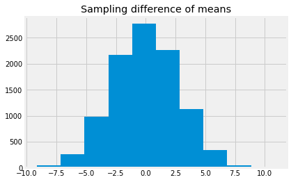
In the permutation test we simulate a ideal (null) world in which there is no average difference between the numbers in the two groups. We do this by pooling the beer and water numbers, shuffling them, and then making fake beer and water groups when we know, from the shuffling, that the average difference will, in the long run, be zero. By doing this shuffle, sample step many times we build up the distribution of the average difference. This is the sampling distribution of the mean difference:

pooled = np.append(beer_activated, water_activated)
n_iters = 10000
fake_differences = np.zeros(n_iters)
for i in np.arange(n_iters):
    np.random.shuffle(pooled)
    fake_differences[i] = np.mean(pooled[:25]) - np.mean(pooled[25:])

plt.hist(fake_differences)
plt.title('Sampling difference of means');

We can work out the proportion of the sampling distribution that is greater than or equal to the observed value, to get an estimate of the probability of the observed value, if we are in fact in the null (ideal) world:

permutation_p = np.count_nonzero(
    fake_differences >= observed_difference)/ n_iters
permutation_p

0.0583

Remember that the standard deviation is a measure of the spread of a distribution.

sampling_sd = np.std(fake_differences)
sampling_sd

2.7544559015909003

We can use the standard deviation as unit of distance in the distribution.

A way of getting an idea of how extreme the observed value is, is to ask how many standard deviations the observed value is from the center of the distribution, which is zero.

like_t = observed_difference / sampling_sd
like_t

1.6095132729381358

Notice the variable name like_t. This number is rather like the famous t statistic.

The difference between this like_t value and the t statistic is that the t statistic is the observed difference divided by another estimate of the standard deviation of the sampling distribution. Specifically it is an estimate that relies on the assumption that the beer_activated and water_activated numbers come from a simple bell-shaped normal distribution.

The specific calculation relies on calculating the prediction errors when we use the mean from each group as the prediction for the values in the group.

beer_errors = beer_activated - np.mean(beer_activated)
water_errors = water_activated - np.mean(water_activated)
all_errors = np.append(beer_errors, water_errors)

The estimate for the standard deviation of the sampling distribution follows this formula. The derivation of the formula is well outside the scope of the class.

# The t-statistic estimate.
n1 = len(beer_activated)
n2 = len(water_activated)
est_error_sd = np.sqrt(np.sum(all_errors ** 2) / (n1 + n2 - 2))
sampling_sd_estimate = est_error_sd * np.sqrt(1 / n1 + 1 / n2)
sampling_sd_estimate

2.7028390172904366

Notice that this is rather similar to the estimate we got directly from the permutation distribution:

sampling_sd

2.7544559015909003

The t statistic is the observed mean difference divided by the estimate of the standard deviation of the sampling distribution.

t_statistic = observed_difference / sampling_sd_estimate
t_statistic

1.640250605001883

This is the same t statistic value calculated by the independent sample t test routine from Scipy:

from scipy.stats import ttest_ind
t_result = ttest_ind(beer_activated, water_activated)
t_result.statistic

1.6402506050018828

The equivalent probability from a t test is also outside the scope of the course, but, if the data we put into the t test is more or less compatible with a normal distribution, then the matching p value is similar to that of the permutation test.

# The "one-tailed" probability from the t-test.
t_result.pvalue / 2

0.054302080886695414

# The permutation p value is very similar.
permutation_p

0.0583

The permutation test is more general than the t test, because the t test relies on the assumption that the numbers come from a normal distribution, but the permutation test does not.