4.1 Introduction to data frames
Introduction to data frames
Pandas is a Python package that implements data frames, and functions that operate on data frames.
# Load the Pands data science library, call it 'pd'
import pandas as pd
We will also use the usual Numpy array library:
# Load the Numpy array library, call it 'np'
import numpy as np
Data frames and series
We start by loading data from a Comma Separated Value file (CSV file). If you are running on your laptop, you should download the gender_stats.csv file to the same directory as this notebook.
See the gender statistics description page for more detail on the dataset.
# Load the data file
gender_data = pd.read_csv('gender_stats.csv')
This is our usual assignment statement. The LHS is gender_data, the variable name. The RHS is an expression, that returns a value.
What type of value does it return?
type(gender_data)
pandas.core.frame.DataFrame
Pandas integrates with the Notebook, so, if you display a data frame in the notebook, it does a nice display of rows and columns.
gender_data
| country_name | country_code | fert_rate | gdp_us_billion | health_exp_per_cap | health_exp_pub | prim_ed_girls | mat_mort_ratio | population | |
|---|---|---|---|---|---|---|---|---|---|
| 0 | Aruba | ABW | 1.663250 | NaN | NaN | NaN | 48.721939 | NaN | 0.103744 |
| 1 | Afghanistan | AFG | 4.954500 | 19.961015 | 161.138034 | 2.834598 | 40.109708 | 444.00 | 32.715838 |
| 2 | Angola | AGO | 6.123000 | 111.936542 | 254.747970 | 2.447546 | NaN | 501.25 | 26.937545 |
| 3 | Albania | ALB | 1.769250 | 12.327586 | 574.202694 | 2.836021 | 47.201082 | 29.25 | 2.888280 |
| 4 | Andorra | AND | NaN | 3.197538 | 4421.224933 | 7.260281 | 47.123345 | NaN | 0.079547 |
| 5 | United Arab Emirates | ARE | 1.793000 | 375.027082 | 2202.407569 | 2.581168 | 48.789260 | 6.00 | 9.080299 |
| 6 | Argentina | ARG | 2.328000 | 550.980968 | 1148.256142 | 2.782216 | 48.915810 | 53.75 | 42.976675 |
| 7 | Armenia | ARM | 1.545500 | 10.885362 | 348.663884 | 1.916016 | 46.782180 | 27.25 | 2.904683 |
| 8 | American Samoa | ASM | NaN | 0.640500 | NaN | NaN | NaN | NaN | 0.055422 |
| 9 | Antigua and Barbuda | ATG | 2.082000 | 1.298213 | 1152.493656 | 3.676514 | 48.291463 | NaN | 0.098872 |
| 10 | Australia | AUS | 1.861500 | 1422.994116 | 4256.058988 | 6.292381 | 48.576707 | 6.00 | 23.444560 |
| 11 | Austria | AUT | 1.455000 | 407.494276 | 4930.298893 | 8.504276 | 48.556078 | 4.00 | 8.566294 |
| 12 | Azerbaijan | AZE | 1.980000 | 62.003001 | 956.709718 | 1.197249 | 46.157363 | 25.25 | 9.531856 |
| 13 | Burundi | BDI | 5.992250 | 2.876978 | 59.693830 | 4.433749 | 50.481971 | 747.25 | 9.907015 |
| 14 | Belgium | BEL | 1.755000 | 494.221836 | 4297.838005 | 8.221003 | 48.864675 | 7.00 | 11.228495 |
| 15 | Benin | BEN | 4.806750 | 8.778151 | 83.726190 | 2.206916 | 47.211127 | 417.50 | 10.293715 |
| 16 | Burkina Faso | BFA | 5.564500 | 11.753054 | 87.143009 | 3.021246 | 48.217520 | 384.25 | 17.597395 |
| 17 | Bangladesh | BGD | 2.193250 | 174.545099 | 85.968844 | 0.860447 | 50.460564 | 194.75 | 159.371214 |
| 18 | Bulgaria | BGR | 1.510000 | 53.797612 | 1266.857003 | 4.243437 | 48.310802 | 10.75 | 7.220151 |
| 19 | Bahrain | BHR | 2.065250 | 32.004011 | 2030.158316 | 2.976386 | 49.116838 | 15.25 | 1.349810 |
| 20 | Bahamas, The | BHS | 1.877250 | 8.688000 | 1727.128385 | 3.308626 | NaN | 81.50 | 0.381904 |
| 21 | Bosnia and Herzegovina | BIH | 1.267000 | 17.323327 | 941.504655 | 6.841021 | 48.634905 | 11.75 | 3.574396 |
| 22 | Belarus | BLR | 1.677000 | 64.782942 | 986.236757 | 3.876601 | 48.685741 | 4.00 | 9.480348 |
| 23 | Belize | BLZ | 2.594750 | 1.680325 | 471.967465 | 3.744844 | 48.317238 | 29.25 | 0.351764 |
| 24 | Bermuda | BMU | 1.617500 | 5.555624 | NaN | NaN | 48.423588 | NaN | 0.065101 |
| 25 | Bolivia | BOL | 2.995250 | 31.509324 | 381.007594 | 4.192031 | 48.464175 | 218.25 | 10.562803 |
| 26 | Brazil | BRA | 1.795250 | 2198.765606 | 1303.199104 | 3.773473 | 47.784577 | 49.50 | 204.159544 |
| 27 | Barbados | BRB | 1.792250 | 4.413080 | 1062.840088 | 4.828680 | 48.878181 | 28.00 | 0.283338 |
| 28 | Brunei Darussalam | BRN | 1.884000 | 15.719223 | 1795.924160 | 2.335194 | 48.523699 | 23.75 | 0.411581 |
| 29 | Bhutan | BTN | 2.061250 | 1.975145 | 277.526670 | 2.706908 | 49.572296 | 161.75 | 0.775905 |
| ... | ... | ... | ... | ... | ... | ... | ... | ... | ... |
| 186 | Turks and Caicos Islands | TCA | NaN | NaN | NaN | NaN | 48.846884 | NaN | 0.033703 |
| 187 | Chad | TCD | 6.211000 | 11.945942 | 69.904561 | 1.725194 | 42.929245 | 892.25 | 13.574024 |
| 188 | Togo | TGO | 4.620000 | 4.183610 | 71.263825 | 2.037809 | 48.270471 | 380.75 | 7.230904 |
| 189 | Thailand | THA | 1.516750 | 406.136904 | 581.927487 | 3.183842 | 48.213034 | 21.00 | 68.384986 |
| 190 | Tajikistan | TJK | 3.495750 | 8.036228 | 169.745970 | 1.976367 | 48.260680 | 33.25 | 8.363844 |
| 191 | Turkmenistan | TKM | 2.313750 | 37.973096 | 288.572644 | 1.349303 | 48.906879 | 43.50 | 5.465637 |
| 192 | Timor-Leste | TLS | 5.797750 | 1.361430 | 98.577296 | 1.140440 | 48.337367 | 240.25 | 1.212718 |
| 193 | Tonga | TON | 3.745750 | 0.439179 | 250.962504 | 3.987285 | 47.697931 | 129.25 | 0.105909 |
| 194 | Trinidad and Tobago | TTO | 1.782750 | 24.570947 | 1778.148073 | 3.071370 | NaN | 63.25 | 1.353877 |
| 195 | Tunisia | TUN | 2.140000 | 44.824374 | 782.950522 | 4.118771 | 48.142132 | 63.25 | 11.144409 |
| 196 | Turkey | TUR | 2.078000 | 895.175577 | 997.374772 | 4.189521 | 48.789477 | 17.50 | 77.034345 |
| 197 | Tuvalu | TUV | NaN | 0.036470 | 563.500592 | 15.506929 | 47.472414 | NaN | 0.010910 |
| 198 | Tanzania | TZA | 5.181250 | 44.935542 | 131.704162 | 2.648609 | 50.666580 | 429.50 | 52.281324 |
| 199 | Uganda | UGA | 5.822500 | 25.941461 | 132.892684 | 2.014349 | 50.099485 | 366.50 | 38.865339 |
| 200 | Ukraine | UKR | 1.510250 | 135.379275 | 628.579254 | 3.960185 | 48.984198 | 24.25 | 45.302704 |
| 201 | Uruguay | URY | 2.027000 | 54.345132 | 1721.507752 | 6.044403 | 48.295555 | 15.50 | 3.419977 |
| 202 | United States | USA | 1.860875 | 17369.124600 | 9060.068657 | 8.121961 | 48.758830 | 14.00 | 318.558175 |
| 203 | Uzbekistan | UZB | 2.372750 | 61.340649 | 334.476754 | 3.118842 | 48.387434 | 37.00 | 30.784500 |
| 204 | St. Vincent and the Grenadines | VCT | 1.986000 | 0.730107 | 775.803386 | 4.365757 | 48.536415 | 45.75 | 0.109421 |
| 205 | Venezuela, RB | VEN | 2.378250 | 376.146268 | 896.815314 | 1.587088 | 48.400934 | 97.00 | 30.734524 |
| 206 | British Virgin Islands | VGB | NaN | NaN | NaN | NaN | 47.581520 | NaN | 0.029585 |
| 207 | Virgin Islands (U.S.) | VIR | 1.760000 | 3.812000 | NaN | NaN | NaN | NaN | 0.104141 |
| 208 | Vietnam | VNM | 1.959500 | 181.820736 | 368.374550 | 3.779501 | 48.021053 | 54.75 | 90.742400 |
| 209 | Vanuatu | VUT | 3.364750 | 0.782876 | 125.568712 | 3.689874 | 47.301617 | 82.50 | 0.258896 |
| 210 | Samoa | WSM | 4.118250 | 0.799887 | 366.353096 | 5.697059 | 48.350049 | 54.75 | 0.192225 |
| 211 | Kosovo | XKX | 2.142500 | 6.804620 | NaN | NaN | NaN | NaN | 1.813820 |
| 212 | Yemen, Rep. | YEM | 4.225750 | 36.819337 | 207.949700 | 1.417836 | 44.470076 | 399.75 | 26.246608 |
| 213 | South Africa | ZAF | 2.375250 | 345.209888 | 1123.142656 | 4.241441 | 48.516298 | 143.75 | 54.177209 |
| 214 | Zambia | ZMB | 5.394250 | 24.280990 | 185.556359 | 2.687290 | 49.934484 | 233.75 | 15.633220 |
| 215 | Zimbabwe | ZWE | 3.943000 | 15.495514 | 115.519881 | 2.695188 | 49.529875 | 398.00 | 15.420964 |
216 rows × 9 columns
The data frame has rows and columns. Like other Python objects, it has attributes. These are pieces of data associated with the data frame. You have already seen methods, which are functions associated with the data frame. You can access attributes in the same way as you access methods, by typing the variable name, followed by a dot ., followed by the attribute name.
For example, one attribute of the data frame, is the shape:
gender_data.shape
(216, 9)
Another attribute is columns. This has the column names. For
example, here is a good way of quickly seeing the column names
for a data frame:
gender_data.columns
Index(['country_name', 'country_code', 'fert_rate', 'gdp_us_billion',
       'health_exp_per_cap', 'health_exp_pub', 'prim_ed_girls',
       'mat_mort_ratio', 'population'],
      dtype='object')
You need more information about what these column names refer to. Here are the longer descriptions from the original data source (link above):
fert_rate: Fertility rate, total (births per woman).gdp_us_billion: GDP (in current US \$ billions).health_exp_per_cap: Health expenditure per capita, PPP (constant 2011 international \$).health_exp_pub: Health expenditure, public (% of GDP).prim_ed_girls: Primary education, pupils (% female).mat_mort_ratio: Maternal mortality ratio (modeled estimate, per 100,000 live births).population: Population, total.
You have just seen array slicing (in Selecting with arrays. You remember that array slicing uses square brackets. Data frames also allow slicing. For example, we often want to get all the data for a single column of the data frame. To do this, we use the same square bracket notation as we use for array slicing, with the name of the column inside the square brackets.
gdp = gender_data['gdp_us_billion']
What type of thing is this column of data?
type(gdp)
pandas.core.series.Series
Here are the values for gdp. You will notice that these are the
same values you saw in the “gdp_us_billion” column when you displayed the whole
data frame.
gdp
0               NaN
1         19.961015
2        111.936542
3         12.327586
4          3.197538
5        375.027082
6        550.980968
7         10.885362
8          0.640500
9          1.298213
10      1422.994116
11       407.494276
12        62.003001
13         2.876978
14       494.221836
15         8.778151
16        11.753054
17       174.545099
18        53.797612
19        32.004011
20         8.688000
21        17.323327
22        64.782942
23         1.680325
24         5.555624
25        31.509324
26      2198.765606
27         4.413080
28        15.719223
29         1.975145
           ...
186             NaN
187       11.945942
188        4.183610
189      406.136904
190        8.036228
191       37.973096
192        1.361430
193        0.439179
194       24.570947
195       44.824374
196      895.175577
197        0.036470
198       44.935542
199       25.941461
200      135.379275
201       54.345132
202    17369.124600
203       61.340649
204        0.730107
205      376.146268
206             NaN
207        3.812000
208      181.820736
209        0.782876
210        0.799887
211        6.804620
212       36.819337
213      345.209888
214       24.280990
215       15.495514
Name: gdp_us_billion, Length: 216, dtype: float64
Missing values and NaN
Looking at the values of gdp (and therefore, the values of the
gdp_us_billion column of gender_data, we see that some of the values are
NaN, which means Not a Number. Pandas uses this marker to indicate values
that are not available, or missing data.
Numpy does not like to calculate with NaN values. Here is Numpy trying to
calculate the median of the gdp values.
np.median(gdp)
/Users/mb312/Library/Python/3.7/lib/python/site-packages/numpy/lib/function_base.py:3250: RuntimeWarning: Invalid value encountered in median
  r = func(a, **kwargs)
nan
Notice the warning about an invalid value.
Numpy recognizes that one or more values are NaN and refuses to guess what to do, when calculating the median.
You saw from the shape above that gender_data has 263 rows. We can use the
general Python len function, to see how many elements there are in gdp.
len(gdp)
216
As expected, it has the same number of elements as there are rows in gender_data.
The count method of the series gives the number of values that are not missing - that is - not NaN.
gdp.count()
200
Plotting with methods
We start with the magic incantation to load the plotting library.
# Load the library for plotting, name it 'plt'
import matplotlib.pyplot as plt
# Display plots inside the notebook.
%matplotlib inline
# Make plots look a little more fancy
plt.style.use('fivethirtyeight')
The gdp variable is a sequence of values, so we can do a histogram on these
values, as we have done histograms on arrays.
plt.hist(gdp);
/Users/mb312/Library/Python/3.7/lib/python/site-packages/numpy/lib/histograms.py:754: RuntimeWarning: invalid value encountered in greater_equal
  keep = (tmp_a >= first_edge)
/Users/mb312/Library/Python/3.7/lib/python/site-packages/numpy/lib/histograms.py:755: RuntimeWarning: invalid value encountered in less_equal
  keep &= (tmp_a <= last_edge)
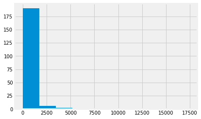
Notice the multiple warnings as Matplotlib tried to calculate the bin widths for the histogram. These warnings result from Matplotlib struggline with NaN values.
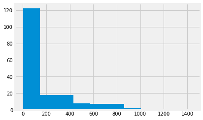
Another way to do the histogram, is to use the hist method of the series.
A method is a function attached to a value. In this case hist is a function attached to a value of type Series.
Using the hist method instead of the plt.hist function can make the code a bit easier to read. The method also has the advantage that it discards the NaN values, by default, so it does not generate the same warnings.
gdp.hist();

Now we have had a look at the GDP values, we will look at the
values for the mat_mort_ratio column. These are the numbers
of women who die in childbirth for every 100,000 births.
mmr = gender_data['mat_mort_ratio']
mmr
0         NaN
1      444.00
2      501.25
3       29.25
4         NaN
5        6.00
6       53.75
7       27.25
8         NaN
9         NaN
10       6.00
11       4.00
12      25.25
13     747.25
14       7.00
15     417.50
16     384.25
17     194.75
18      10.75
19      15.25
20      81.50
21      11.75
22       4.00
23      29.25
24        NaN
25     218.25
26      49.50
27      28.00
28      23.75
29     161.75
        ...
186       NaN
187    892.25
188    380.75
189     21.00
190     33.25
191     43.50
192    240.25
193    129.25
194     63.25
195     63.25
196     17.50
197       NaN
198    429.50
199    366.50
200     24.25
201     15.50
202     14.00
203     37.00
204     45.75
205     97.00
206       NaN
207       NaN
208     54.75
209     82.50
210     54.75
211       NaN
212    399.75
213    143.75
214    233.75
215    398.00
Name: mat_mort_ratio, Length: 216, dtype: float64
mmr.hist();
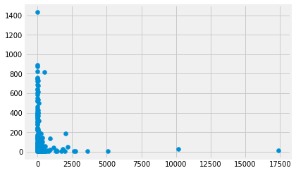
We are interested in the relationship of gpp and mmr. Maybe richer countries have better health care, and fewer maternal deaths.
Here is a plot, using the standard Matplotlib scatter
function.
plt.scatter(gdp, mmr);
We can do the same plot using the plot.scatter method on the data frame. In that case, we specify the column names that should go on the x and the y axes.
gender_data.plot.scatter('gdp_us_billion', 'mat_mort_ratio');
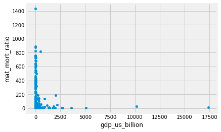
An advantage of doing it this way is that we get the column names on the x and y axes by default.
Showing the top 5 values with the head method
We have already seen that Pandas will display the data frame with nice formatting. If the data frame is long, it will display only the first few and the last few rows:
gender_data
| country_name | country_code | fert_rate | gdp_us_billion | health_exp_per_cap | health_exp_pub | prim_ed_girls | mat_mort_ratio | population | |
|---|---|---|---|---|---|---|---|---|---|
| 0 | Aruba | ABW | 1.663250 | NaN | NaN | NaN | 48.721939 | NaN | 0.103744 |
| 1 | Afghanistan | AFG | 4.954500 | 19.961015 | 161.138034 | 2.834598 | 40.109708 | 444.00 | 32.715838 |
| 2 | Angola | AGO | 6.123000 | 111.936542 | 254.747970 | 2.447546 | NaN | 501.25 | 26.937545 |
| 3 | Albania | ALB | 1.769250 | 12.327586 | 574.202694 | 2.836021 | 47.201082 | 29.25 | 2.888280 |
| 4 | Andorra | AND | NaN | 3.197538 | 4421.224933 | 7.260281 | 47.123345 | NaN | 0.079547 |
| 5 | United Arab Emirates | ARE | 1.793000 | 375.027082 | 2202.407569 | 2.581168 | 48.789260 | 6.00 | 9.080299 |
| 6 | Argentina | ARG | 2.328000 | 550.980968 | 1148.256142 | 2.782216 | 48.915810 | 53.75 | 42.976675 |
| 7 | Armenia | ARM | 1.545500 | 10.885362 | 348.663884 | 1.916016 | 46.782180 | 27.25 | 2.904683 |
| 8 | American Samoa | ASM | NaN | 0.640500 | NaN | NaN | NaN | NaN | 0.055422 |
| 9 | Antigua and Barbuda | ATG | 2.082000 | 1.298213 | 1152.493656 | 3.676514 | 48.291463 | NaN | 0.098872 |
| 10 | Australia | AUS | 1.861500 | 1422.994116 | 4256.058988 | 6.292381 | 48.576707 | 6.00 | 23.444560 |
| 11 | Austria | AUT | 1.455000 | 407.494276 | 4930.298893 | 8.504276 | 48.556078 | 4.00 | 8.566294 |
| 12 | Azerbaijan | AZE | 1.980000 | 62.003001 | 956.709718 | 1.197249 | 46.157363 | 25.25 | 9.531856 |
| 13 | Burundi | BDI | 5.992250 | 2.876978 | 59.693830 | 4.433749 | 50.481971 | 747.25 | 9.907015 |
| 14 | Belgium | BEL | 1.755000 | 494.221836 | 4297.838005 | 8.221003 | 48.864675 | 7.00 | 11.228495 |
| 15 | Benin | BEN | 4.806750 | 8.778151 | 83.726190 | 2.206916 | 47.211127 | 417.50 | 10.293715 |
| 16 | Burkina Faso | BFA | 5.564500 | 11.753054 | 87.143009 | 3.021246 | 48.217520 | 384.25 | 17.597395 |
| 17 | Bangladesh | BGD | 2.193250 | 174.545099 | 85.968844 | 0.860447 | 50.460564 | 194.75 | 159.371214 |
| 18 | Bulgaria | BGR | 1.510000 | 53.797612 | 1266.857003 | 4.243437 | 48.310802 | 10.75 | 7.220151 |
| 19 | Bahrain | BHR | 2.065250 | 32.004011 | 2030.158316 | 2.976386 | 49.116838 | 15.25 | 1.349810 |
| 20 | Bahamas, The | BHS | 1.877250 | 8.688000 | 1727.128385 | 3.308626 | NaN | 81.50 | 0.381904 |
| 21 | Bosnia and Herzegovina | BIH | 1.267000 | 17.323327 | 941.504655 | 6.841021 | 48.634905 | 11.75 | 3.574396 |
| 22 | Belarus | BLR | 1.677000 | 64.782942 | 986.236757 | 3.876601 | 48.685741 | 4.00 | 9.480348 |
| 23 | Belize | BLZ | 2.594750 | 1.680325 | 471.967465 | 3.744844 | 48.317238 | 29.25 | 0.351764 |
| 24 | Bermuda | BMU | 1.617500 | 5.555624 | NaN | NaN | 48.423588 | NaN | 0.065101 |
| 25 | Bolivia | BOL | 2.995250 | 31.509324 | 381.007594 | 4.192031 | 48.464175 | 218.25 | 10.562803 |
| 26 | Brazil | BRA | 1.795250 | 2198.765606 | 1303.199104 | 3.773473 | 47.784577 | 49.50 | 204.159544 |
| 27 | Barbados | BRB | 1.792250 | 4.413080 | 1062.840088 | 4.828680 | 48.878181 | 28.00 | 0.283338 |
| 28 | Brunei Darussalam | BRN | 1.884000 | 15.719223 | 1795.924160 | 2.335194 | 48.523699 | 23.75 | 0.411581 |
| 29 | Bhutan | BTN | 2.061250 | 1.975145 | 277.526670 | 2.706908 | 49.572296 | 161.75 | 0.775905 |
| ... | ... | ... | ... | ... | ... | ... | ... | ... | ... |
| 186 | Turks and Caicos Islands | TCA | NaN | NaN | NaN | NaN | 48.846884 | NaN | 0.033703 |
| 187 | Chad | TCD | 6.211000 | 11.945942 | 69.904561 | 1.725194 | 42.929245 | 892.25 | 13.574024 |
| 188 | Togo | TGO | 4.620000 | 4.183610 | 71.263825 | 2.037809 | 48.270471 | 380.75 | 7.230904 |
| 189 | Thailand | THA | 1.516750 | 406.136904 | 581.927487 | 3.183842 | 48.213034 | 21.00 | 68.384986 |
| 190 | Tajikistan | TJK | 3.495750 | 8.036228 | 169.745970 | 1.976367 | 48.260680 | 33.25 | 8.363844 |
| 191 | Turkmenistan | TKM | 2.313750 | 37.973096 | 288.572644 | 1.349303 | 48.906879 | 43.50 | 5.465637 |
| 192 | Timor-Leste | TLS | 5.797750 | 1.361430 | 98.577296 | 1.140440 | 48.337367 | 240.25 | 1.212718 |
| 193 | Tonga | TON | 3.745750 | 0.439179 | 250.962504 | 3.987285 | 47.697931 | 129.25 | 0.105909 |
| 194 | Trinidad and Tobago | TTO | 1.782750 | 24.570947 | 1778.148073 | 3.071370 | NaN | 63.25 | 1.353877 |
| 195 | Tunisia | TUN | 2.140000 | 44.824374 | 782.950522 | 4.118771 | 48.142132 | 63.25 | 11.144409 |
| 196 | Turkey | TUR | 2.078000 | 895.175577 | 997.374772 | 4.189521 | 48.789477 | 17.50 | 77.034345 |
| 197 | Tuvalu | TUV | NaN | 0.036470 | 563.500592 | 15.506929 | 47.472414 | NaN | 0.010910 |
| 198 | Tanzania | TZA | 5.181250 | 44.935542 | 131.704162 | 2.648609 | 50.666580 | 429.50 | 52.281324 |
| 199 | Uganda | UGA | 5.822500 | 25.941461 | 132.892684 | 2.014349 | 50.099485 | 366.50 | 38.865339 |
| 200 | Ukraine | UKR | 1.510250 | 135.379275 | 628.579254 | 3.960185 | 48.984198 | 24.25 | 45.302704 |
| 201 | Uruguay | URY | 2.027000 | 54.345132 | 1721.507752 | 6.044403 | 48.295555 | 15.50 | 3.419977 |
| 202 | United States | USA | 1.860875 | 17369.124600 | 9060.068657 | 8.121961 | 48.758830 | 14.00 | 318.558175 |
| 203 | Uzbekistan | UZB | 2.372750 | 61.340649 | 334.476754 | 3.118842 | 48.387434 | 37.00 | 30.784500 |
| 204 | St. Vincent and the Grenadines | VCT | 1.986000 | 0.730107 | 775.803386 | 4.365757 | 48.536415 | 45.75 | 0.109421 |
| 205 | Venezuela, RB | VEN | 2.378250 | 376.146268 | 896.815314 | 1.587088 | 48.400934 | 97.00 | 30.734524 |
| 206 | British Virgin Islands | VGB | NaN | NaN | NaN | NaN | 47.581520 | NaN | 0.029585 |
| 207 | Virgin Islands (U.S.) | VIR | 1.760000 | 3.812000 | NaN | NaN | NaN | NaN | 0.104141 |
| 208 | Vietnam | VNM | 1.959500 | 181.820736 | 368.374550 | 3.779501 | 48.021053 | 54.75 | 90.742400 |
| 209 | Vanuatu | VUT | 3.364750 | 0.782876 | 125.568712 | 3.689874 | 47.301617 | 82.50 | 0.258896 |
| 210 | Samoa | WSM | 4.118250 | 0.799887 | 366.353096 | 5.697059 | 48.350049 | 54.75 | 0.192225 |
| 211 | Kosovo | XKX | 2.142500 | 6.804620 | NaN | NaN | NaN | NaN | 1.813820 |
| 212 | Yemen, Rep. | YEM | 4.225750 | 36.819337 | 207.949700 | 1.417836 | 44.470076 | 399.75 | 26.246608 |
| 213 | South Africa | ZAF | 2.375250 | 345.209888 | 1123.142656 | 4.241441 | 48.516298 | 143.75 | 54.177209 |
| 214 | Zambia | ZMB | 5.394250 | 24.280990 | 185.556359 | 2.687290 | 49.934484 | 233.75 | 15.633220 |
| 215 | Zimbabwe | ZWE | 3.943000 | 15.495514 | 115.519881 | 2.695188 | 49.529875 | 398.00 | 15.420964 |
216 rows × 9 columns
Notice the ... in the center of this listing, to show that it has not printed some rows.
Sometimes we do not want to see all these rows, but only - say - the top five rows. The head method of the data frame is a useful way to do this:
gender_data.head()
| country_name | country_code | fert_rate | gdp_us_billion | health_exp_per_cap | health_exp_pub | prim_ed_girls | mat_mort_ratio | population | |
|---|---|---|---|---|---|---|---|---|---|
| 0 | Aruba | ABW | 1.66325 | NaN | NaN | NaN | 48.721939 | NaN | 0.103744 |
| 1 | Afghanistan | AFG | 4.95450 | 19.961015 | 161.138034 | 2.834598 | 40.109708 | 444.00 | 32.715838 |
| 2 | Angola | AGO | 6.12300 | 111.936542 | 254.747970 | 2.447546 | NaN | 501.25 | 26.937545 |
| 3 | Albania | ALB | 1.76925 | 12.327586 | 574.202694 | 2.836021 | 47.201082 | 29.25 | 2.888280 |
| 4 | Andorra | AND | NaN | 3.197538 | 4421.224933 | 7.260281 | 47.123345 | NaN | 0.079547 |
The Series also has a head method, that does the same thing:
gdp.head()
0           NaN
1     19.961015
2    111.936542
3     12.327586
4      3.197538
Name: gdp_us_billion, dtype: float64
Selecting rows
We often want to select rows from the data frame that match some criterion.
Say we want to select the rows corresponding the countries with a high GDP.
Looking at the histogram of gdp above, we could try this as a threshold to
identify high GDP countries.
high_gdp = gdp > 1000
high_gdp.head()
0    False
1    False
2    False
3    False
4    False
Name: gdp_us_billion, dtype: bool
type(high_gdp)
pandas.core.series.Series
Notice that high_gdp is a Boolean series, like the Boolean arrays you have
already seen. It has True for elements corresponding to countries with gdp
value greater than 1000 and False otherwise.
We can use this Boolean series to select rows from the data frame.
Remember indexing. When we follow a name of something, like an array or series or data frame, with an open square bracket, this means we are trying to get data from the array or Series. The stuff inside the square brackets says what we want.
When we put our Boolean series inside the square brackets, it works like this:
rich_gender_data = gender_data[high_gdp]
rich_gender_data
| country_name | country_code | fert_rate | gdp_us_billion | health_exp_per_cap | health_exp_pub | prim_ed_girls | mat_mort_ratio | population | |
|---|---|---|---|---|---|---|---|---|---|
| 10 | Australia | AUS | 1.861500 | 1422.994116 | 4256.058988 | 6.292381 | 48.576707 | 6.00 | 23.444560 |
| 26 | Brazil | BRA | 1.795250 | 2198.765606 | 1303.199104 | 3.773473 | 47.784577 | 49.50 | 204.159544 |
| 32 | Canada | CAN | 1.600300 | 1708.473627 | 4616.539134 | 7.546247 | 48.808926 | 7.25 | 35.517119 |
| 35 | China | CHN | 1.558750 | 10182.790479 | 657.748859 | 3.015530 | 46.297964 | 28.75 | 1364.446000 |
| 49 | Germany | DEU | 1.450000 | 3601.226158 | 4909.659884 | 8.542615 | 48.568695 | 6.25 | 81.281645 |
| 58 | Spain | ESP | 1.307500 | 1299.724261 | 2963.832825 | 6.545739 | 48.722231 | 5.00 | 46.553128 |
| 63 | France | FRA | 2.005000 | 2647.649725 | 4387.835406 | 8.920420 | 48.772050 | 8.75 | 66.302099 |
| 67 | United Kingdom | GBR | 1.842500 | 2768.864417 | 3357.983675 | 7.720655 | 48.791809 | 9.25 | 64.641557 |
| 88 | India | IND | 2.449250 | 2019.005411 | 241.572477 | 1.292666 | 49.497234 | 185.25 | 1293.742537 |
| 94 | Italy | ITA | 1.390000 | 2005.983980 | 3266.984094 | 6.984374 | 48.407573 | 4.00 | 60.378795 |
| 97 | Japan | JPN | 1.430000 | 5106.024760 | 3687.126279 | 8.496074 | 48.744199 | 5.75 | 127.297102 |
| 104 | Korea, Rep. | KOR | 1.232000 | 1346.751162 | 2385.447251 | 3.915606 | 48.023388 | 12.00 | 50.727212 |
| 124 | Mexico | MEX | 2.257000 | 1188.802780 | 1081.208948 | 3.225839 | 48.906296 | 40.00 | 124.203450 |
| 164 | Russian Federation | RUS | 1.724500 | 1822.691700 | 1755.506635 | 3.731354 | 48.968070 | 25.25 | 143.793504 |
| 202 | United States | USA | 1.860875 | 17369.124600 | 9060.068657 | 8.121961 | 48.758830 | 14.00 | 318.558175 |
type(rich_gender_data)
pandas.core.frame.DataFrame
rich_gender_data is a new data frame, that is a subset of the original
gender_data frame. It contains only the rows where the GDP value is greater
than 1000 billion dollars. Check the display of rich_gender_data above to
confirm that the values in the gdp_us_billion column are all greater than
1000.
We can do a scatter plot of GDP values against maternal mortality rate, and we find, oddly, that for rich countries, there is little relationship between GDP and maternal mortality.
rich_gender_data.plot.scatter('gdp_us_billion', 'mat_mort_ratio')
<matplotlib.axes._subplots.AxesSubplot at 0x1150beb90>
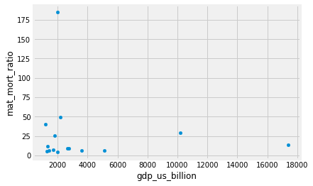
One thing that stands out is the very high value at around 180. Which country does this refer to? We can use sorting to find out.
Sorting data frames
Data frames have a method sort_value. This returns a new data frame with the
rows sorted by the values in the column we specify.
Here are the first five rows of the data frame of the rich countries:
rich_gender_data.head()
| country_name | country_code | fert_rate | gdp_us_billion | health_exp_per_cap | health_exp_pub | prim_ed_girls | mat_mort_ratio | population | |
|---|---|---|---|---|---|---|---|---|---|
| 10 | Australia | AUS | 1.86150 | 1422.994116 | 4256.058988 | 6.292381 | 48.576707 | 6.00 | 23.444560 |
| 26 | Brazil | BRA | 1.79525 | 2198.765606 | 1303.199104 | 3.773473 | 47.784577 | 49.50 | 204.159544 |
| 32 | Canada | CAN | 1.60030 | 1708.473627 | 4616.539134 | 7.546247 | 48.808926 | 7.25 | 35.517119 |
| 35 | China | CHN | 1.55875 | 10182.790479 | 657.748859 | 3.015530 | 46.297964 | 28.75 | 1364.446000 |
| 49 | Germany | DEU | 1.45000 | 3601.226158 | 4909.659884 | 8.542615 | 48.568695 | 6.25 | 81.281645 |
We are interested to find which of these richer countries has a high maternal mortality ratio. To do this, we can make a new data frame where the rows are sorted by the values in the
mat_mort_ratio column:
rich_by_mmr = rich_gender_data.sort_values('mat_mort_ratio')
rich_by_mmr.head()
| country_name | country_code | fert_rate | gdp_us_billion | health_exp_per_cap | health_exp_pub | prim_ed_girls | mat_mort_ratio | population | |
|---|---|---|---|---|---|---|---|---|---|
| 94 | Italy | ITA | 1.3900 | 2005.983980 | 3266.984094 | 6.984374 | 48.407573 | 4.00 | 60.378795 |
| 58 | Spain | ESP | 1.3075 | 1299.724261 | 2963.832825 | 6.545739 | 48.722231 | 5.00 | 46.553128 |
| 97 | Japan | JPN | 1.4300 | 5106.024760 | 3687.126279 | 8.496074 | 48.744199 | 5.75 | 127.297102 |
| 10 | Australia | AUS | 1.8615 | 1422.994116 | 4256.058988 | 6.292381 | 48.576707 | 6.00 | 23.444560 |
| 49 | Germany | DEU | 1.4500 | 3601.226158 | 4909.659884 | 8.542615 | 48.568695 | 6.25 | 81.281645 |
Notice that the rows are in ascending order of mat_mort_ratio. To find the countries with high maternal mortality, we might prefer to sort in descending order. As usual you can explore how
you might do this by looking at the help for the sort_values method with:
rich_by_mmr.sort_values?
in a new cell. If you do that, you discover the ascending argument, that
you can use like this:
rich_by_descending_mmr = rich_gender_data.sort_values('mat_mort_ratio', ascending=False)
rich_by_descending_mmr.head()
| country_name | country_code | fert_rate | gdp_us_billion | health_exp_per_cap | health_exp_pub | prim_ed_girls | mat_mort_ratio | population | |
|---|---|---|---|---|---|---|---|---|---|
| 88 | India | IND | 2.44925 | 2019.005411 | 241.572477 | 1.292666 | 49.497234 | 185.25 | 1293.742537 |
| 26 | Brazil | BRA | 1.79525 | 2198.765606 | 1303.199104 | 3.773473 | 47.784577 | 49.50 | 204.159544 |
| 124 | Mexico | MEX | 2.25700 | 1188.802780 | 1081.208948 | 3.225839 | 48.906296 | 40.00 | 124.203450 |
| 35 | China | CHN | 1.55875 | 10182.790479 | 657.748859 | 3.015530 | 46.297964 | 28.75 | 1364.446000 |
| 164 | Russian Federation | RUS | 1.72450 | 1822.691700 | 1755.506635 | 3.731354 | 48.968070 | 25.25 | 143.793504 |
As you might have guessed by now, Series also have a sort_values method.
For a Series, you don’t have to specify the column to sort from, because you
are using the Series values.
rich_mmr = rich_gender_data['mat_mort_ratio']
type(rich_mmr)
pandas.core.series.Series
rich_mmr.sort_values(ascending=False)
88     185.25
26      49.50
124     40.00
35      28.75
164     25.25
202     14.00
104     12.00
67       9.25
63       8.75
32       7.25
49       6.25
10       6.00
97       5.75
58       5.00
94       4.00
Name: mat_mort_ratio, dtype: float64
Calculation on data frames
We can calculate with Pandas Series, just as we can with arrays.
For example, now we know that India has both a high GDP, and a high maternal mortality ratio, we wonder whether this is because India also has a large population, and therefore, relatively little money per person to spend on health care.
So, we would like know the GDP per capita. Luckily the data frame as a column “population”:
rich_population = rich_by_descending_mmr["population"]
rich_population
88     1293.742537
26      204.159544
124     124.203450
35     1364.446000
164     143.793504
202     318.558175
104      50.727212
67       64.641557
63       66.302099
32       35.517119
49       81.281645
10       23.444560
97      127.297102
58       46.553128
94       60.378795
Name: population, dtype: float64
We can divide the GDP by the population in millions to get US billion dollars per million population.
This works exactly as it does for arrays:
rich_gdp = rich_by_descending_mmr["gdp_us_billion"]
rich_gdp
88      2019.005411
26      2198.765606
124     1188.802780
35     10182.790479
164     1822.691700
202    17369.124600
104     1346.751162
67      2768.864417
63      2647.649725
32      1708.473627
49      3601.226158
10      1422.994116
97      5106.024760
58      1299.724261
94      2005.983980
Name: gdp_us_billion, dtype: float64
gdp_per_million = rich_gdp / rich_population
gdp_per_million
88      1.560593
26     10.769840
124     9.571415
35      7.462949
164    12.675758
202    54.524184
104    26.548890
67     42.834123
63     39.933121
32     48.102821
49     44.305528
10     60.696133
97     40.111084
58     27.919161
94     33.223319
dtype: float64
Notice that the result is elementwise division, that is Python divides
each element in rich_gdp by the corresponding element in
rich_population.
Remember that India is the first country in the rich_by_descending_mmr
data frame. It also has by far the lowest GDP per million population of
any of this selection of rich countries. Here’s a plot of
gdp_per_million against the corresponding values in mat_mort_ratio:
plt.scatter(gdp_per_million, rich_by_descending_mmr['mat_mort_ratio'])
<matplotlib.collections.PathCollection at 0x114251dd0>
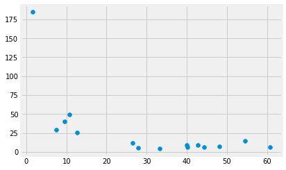
It does look as if low income per person predisposes to high maternal mortality.