\(\newcommand{L}[1]{\| #1 \|}\newcommand{VL}[1]{\L{ \vec{#1} }}\newcommand{R}[1]{\operatorname{Re}\,(#1)}\newcommand{I}[1]{\operatorname{Im}\, (#1)}\)
Schooling and fertility
Here we are analyzing this dataset from the World Bank on gender and inequality:
You can download the data yourself as a zip file from that site, but to make your life a little easier, I’ve made a link to the extracted data file:
Download this file to the same directory as your Jupyter Notebook.
>>> # Import Pandas with its usual short name
>>> import pandas as pd
Load the Comma Separated Value text file into Pandas as a data frame:
>>> df = pd.read_csv('Gender_StatsData.csv')
This is a slightly clumsy-looking data frame, because it has years for columns, and variables for rows, where there are 630 variables for each country. So there are 630 rows * the number of countries. To investigate, we first look at the column names:
>>> df.columns
Index(['"Country Name"', 'Country Code', 'Indicator Name', 'Indicator Code',
       '1960', '1961', '1962', '1963', '1964', '1965', '1966', '1967', '1968',
       '1969', '1970', '1971', '1972', '1973', '1974', '1975', '1976', '1977',
       '1978', '1979', '1980', '1981', '1982', '1983', '1984', '1985', '1986',
       '1987', '1988', '1989', '1990', '1991', '1992', '1993', '1994', '1995',
       '1996', '1997', '1998', '1999', '2000', '2001', '2002', '2003', '2004',
       '2005', '2006', '2007', '2008', '2009', '2010', '2011', '2012', '2013',
       '2014', '2015', '2016', '2017', 'Unnamed: 62'],
      dtype='object')
Next we look at the data frame itself:
>>> df
       "Country Name" Country Code  \
0           Arab World          ARB ...
1           Arab World          ARB ...
2           Arab World          ARB ...
3           Arab World          ARB ...
4           Arab World          ARB ...
5           Arab World          ARB ...
...

[165690 rows x 63 columns]
There are lots of countries here, so to start, let’s look at the variables for the UK.
We get the UK country code from http://www.worldatlas.com/aatlas/ctycodes.htm.
The code is GBR.
>>> # We select only the UK rows
>>> gb = df[df['Country Code'] == 'GBR']
>>> gb
       "Country Name" Country Code  \
158130  United Kingdom          GBR ...
158131  United Kingdom          GBR ...
158132  United Kingdom          GBR ...
158133  United Kingdom          GBR ...
158134  United Kingdom          GBR ...
158135  United Kingdom          GBR ...
...

[630 rows x 63 columns]
Pandas truncates the output to only show a certain number of rows, and only a certain length for the text fields. To investigate further, you can increase these limits to see all 630 rows for the UK, and more of the text for the text fields:
>>> # See more of the text, more rows in the displayed output
>>> pd.options.display.max_colwidth = 80
>>> pd.options.display.max_rows = 700
If you are working in the Notebook, you will now see all of the rows and the whole text field with the variable description.
>>> # This will be different from above when working in the Notebook
>>> gb
       "Country Name" Country Code  \
158130  United Kingdom          GBR ...
158131  United Kingdom          GBR ...
158132  United Kingdom          GBR ...
158133  United Kingdom          GBR ...
158134  United Kingdom          GBR ...
158135  United Kingdom          GBR ...
...

[630 rows x 63 columns]
After scanning through this output, we decide we want to look at these two variables:
SP.ADO.TFRT: Adolescent fertility rate (births per 1,000 women ages 15-19)SE.SCH.LIFE.FE: Expected years of schooling, female
Remember that, for each variable there is one row per country. We have to select the rows corresponding to this variable, for all countries. We do that for both variables we are interested in.
>>> # Put the variables we want into their own data frames
>>> fertility_rate = df[df['Indicator Code'] == 'SP.ADO.TFRT']
>>> age_female_sch = df[df['Indicator Code'] == 'SE.SCH.LIFE.FE']
For convenience, we are going to put the values from these columns back into their own data frame. To do that, we make a new data frame, and fill it with the values from our variables:
>>> # Make a new data frame to store our school and fertility columns
>>> school_fertility = pd.DataFrame(columns=['school', 'fertility'])
>>> school_fertility
Empty DataFrame
Columns: [school, fertility]
Index: []
We fill the empty data frame with the values we selected:
>>> school_fertility['school'] = age_female_sch['2014'].values
>>> school_fertility['fertility'] = fertility_rate['2014'].values
>>> school_fertility
        school   fertility
0    10.993670   48.479108
1          NaN   57.160052
2    16.449970   19.519840
3    11.816701   41.685074
4    13.469607   21.358688
5    13.257181   22.752998
...
We do not have the expected length of schooling for quite a few contries;
these are the rows with NaN in the corresponding columns. “NaN” stands
for Not a Number. We often call these missing values. They can also be
called “NA” for “Not Applicable”. There are some missing values for the
fertility statistic too. For simplicity, we drop rows that have missing
values in either of these two columns:
>>> # Drop the rows with any missing (NaN) values
>>> school_fertility = school_fertility.dropna()
>>> school_fertility
        school   fertility
0    10.993670   48.479108
2    16.449970   19.519840
3    11.816701   41.685074
4    13.469607   21.358688
5    13.257181   22.752998
6    13.280039   23.077289
...
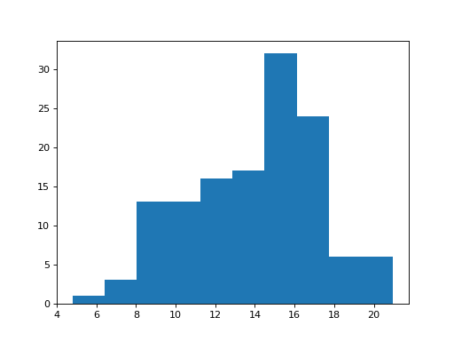
Now we have the data we think we want, we do a quick check for odd values by doing a histogram of each column:
Hint
If running in the IPython console, consider running %matplotlib to enable
interactive plots. If running in the Jupyter Notebook, use %matplotlib
inline.
>>> # Import the plotting library with a memorable name
>>> import matplotlib.pyplot as plt
>>> # Histogram of the school length
>>> plt.hist(school_fertility['school']);
(...)
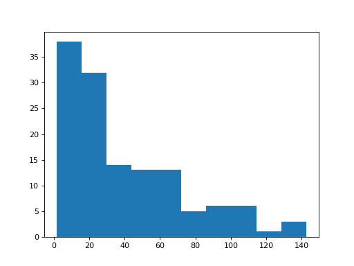
>>> # Histogram of the fertility rate
>>> plt.hist(school_fertility['fertility']);
(...)

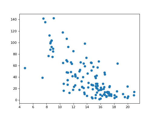
Now to the part we are interested in. We speculate that countries that don’t keep their women in school for long, may have higher adolescent fertility rates. We plot length of schooling on the X axis and fertility rates on the Y axis:
>>> # Scatterplot of school length against fertility rate
>>> plt.scatter(school_fertility['school'], school_fertility['fertility'])
<...>

We save the data frame we made to a file, so we can use these values again. When saving, we drop off the first implicit column, with the case numbers:
>>> school_fertility.to_csv('school_fertility.csv', index=False)
As usual, we make lists for our two sets of numbers:
>>> school = list(school_fertility['school'])
>>> fertility = list(school_fertility['fertility'])
We have speculated that, as the number of years in school goes up, the number of adolescents having children goes down.
Remember What order is best?? If school and fertility are
perfectly arranged, with low values for school going with high values of
fertility, we will get a high list_product:
>>> def list_product(first_list, second_list):
...     product = 0
...     for i in range(len(first_list)):
...         value = first_list[i] * second_list[i]
...         product = product + value
...     return product
So, what do we get for our observed lists?
>>> observed_product = list_product(school, fertility)
What do we compare this to? What is our sampling distribution?
We need our null hypothesis again.
Our null hypothesis is that there is no systematic shared ordering to
school and fertility. Any appearance of shared ordering is just
because of random sampling variation in school and fertility.
We can get an idea of sampling variation by doing something very similar to
what we did in Comparing two groups with permutation testing. We can permute the fertility list to
give a random sample of fertility values. So, here is one trial:
>>> #: The random module
>>> import random
>>> def one_product(list_1, list_2):
...     # We don't want to change list_2, so make a copy
...     new_list_2 = list_2.copy()
...     random.shuffle(new_list_2)
...     return list_product(list_1, new_list_2)
>>> one_product(school, fertility)
75196.897957675363
>>> one_product(school, fertility)
72668.685532226926
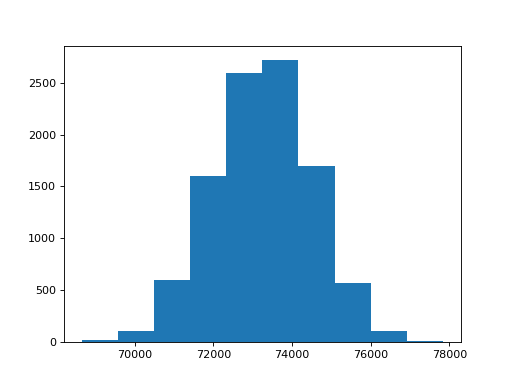
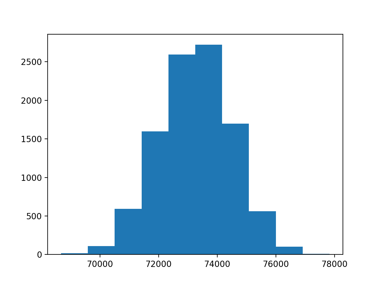
Now let’s build up the sampling distribution:
>>> n_repeats = 10000
>>> sample_products = []
>>> for i in range(n_repeats):
...     product = one_product(school, fertility)
...     sample_products.append(product)
>>> plt.hist(sample_products)
(...)