\(\newcommand{L}[1]{\| #1 \|}\newcommand{VL}[1]{\L{ \vec{#1} }}\newcommand{R}[1]{\operatorname{Re}\,(#1)}\newcommand{I}[1]{\operatorname{Im}\, (#1)}\)
Analyzing Brexit
Every year, the Hansard Society sponsors a survey on political engagement in the UK.
They put topical questions in each survey. For the 2016 / 7 survey, they asked about how people voted in the Brexit referendum.
Luckily, they make the data freely available online for us to analyze.
You can get the data for yourself from the UK Data Service: https://discover.ukdataservice.ac.uk/catalogue/?sn=8183.
To save you a tiny bit of work, I’ve made an unchanged copy of the “tab-delimited” data file for you to download directly. I’ve also made a copy of the document describing the questions they ask and the way that they have recorded the answers in the data file. This is often called the “data dictionary”. It was originally in Rich Text Format, but I have converted to PDF for convenience. It is otherwise identical to the file you will find at the UK Data Service.
Download these files to the working directory for your Jupyter Notebook:
We are going to load this data using the Pandas package for data analysis.
Pandas is a large, powerful package that is very popular for data analysis. You might want to read the Pandas documentation and you will find lots of help with Google searches and the StackOverflow question answer site.
First we import the package, so it is ready to use. Actually we will import it, and also give it a nice short name so we do not have to do much typing to use the package:
>>> import pandas as pd
The data file that you just downloaded should be called
audit_of_political_engagement_14_2017.tab. We load the data file into
memory with Pandas:
>>> # Notice we use "pd" to refer to the Pandas package (see above)
>>> audit_data = pd.read_table('audit_of_political_engagement_14_2017.tab')
We now have something called a “data frame”. This is a table, rather like a spreadsheet, where there is one row per person surveyed, and one column for each question in the survey. The columns have helpful names that you can read about in the data dictionary:
>>> audit_data
      cu041  cu042  cu043  cu044  cu045  cu046  cu047  cu048  cu049  cu0410  \
0         0      0      0      0      1      1      0      0      0       0 ...
1         0      0      0      0      0      0      0      0      0       1 ...
2         0      0      0      0      1      0      0      0      0       0 ...
3         0      0      0      0      1      0      1      0      0       0 ...
4         0      0      0      1      1      0      1      0      0       0 ...
5         1      1      0      0      0      0      0      0      0       0 ...
...

[1771 rows x 370 columns]
The data frame has columns for all the questions listed in the data dictionary:
>>> audit_data.columns
Index(['cu041', 'cu042', 'cu043', 'cu044', 'cu045', 'cu046', 'cu047', 'cu048',
       'cu049', 'cu0410',
       ...
       'intten', 'cx_971_980', 'serial', 'week', 'wts', 'numage', 'weight0',
       'sgrade_grp', 'age_grp', 'region2'],
      dtype='object', length=370)
For the moment, we will focus on two questions labeled cut15
and numage. cut15 is the question about Brexit. The data dictionary
has the variable label “CUT15 - How did you vote on the question ‘Should the
United Kingdom remain a member of the European Union or leave the European
Union’?”. The recorded values run from 1 through 6 and have the following
labels:
Value label information for cut15
Value = 1.0    Label = Remain a member of the European Union
Value = 2.0    Label = Leave the European Union
Value = 3.0    Label = Did not vote
Value = 4.0    Label = Too young
Value = 5.0    Label = Can't remember
Value = 6.0    Label = Refused
We also want the variable numage; this is the age of the respondent in
years.
To reduce clutter, we first make a new data frame that just has the two questions we are interested in:
>>> # Select the age and Brexit vote questions only
>>> brexit_age = audit_data[['numage', 'cut15']]
>>> brexit_age
      numage  cut15
0         37      1
1         55      1
2         71      2
3         37      1
4         42      1
5          0      1
...

[1771 rows x 2 columns]
The variable name cut15 is not very memorable, and we care about
memorable, because good names help to keep our ideas clear as we are working.
We rename the columns from their original names to more memorable ones:
>>> # Rename the columns to be more memorable
>>> brexit_age.columns = ['age', 'brexit']
>>> brexit_age
      age  brexit
0      37       1
1      55       1
2      71       2
3      37       1
4      42       1
5       0       1
...

[1771 rows x 2 columns]
Wait — there’s something odd in those numbers.
We were lucky to spot that, but in any case, we want to check our data before we continue. The first thing we do is make a histogram of the ages.
To do this we first need to load the standard Python plotting library, Matplotlib.
Hint
If running in the IPython console, consider running %matplotlib to enable
interactive plots. If running in the Jupyter Notebook, use %matplotlib
inline.
Remember that we did an “import” for the Pandas package above. Now we import
part of matplotlib, and again, we give it a short memorable name:
>>> import matplotlib.pyplot as plt
Here is a histogram of the respondents’ ages:
>>> plt.hist(brexit_age['age'])
(...)
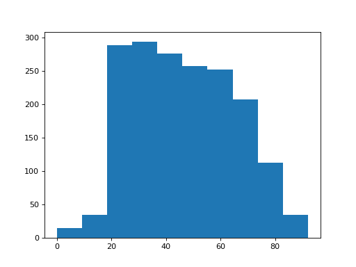
There appear to be a few subjects with age of 0.
It looks as if the survey coders are using the value 0 to mean that the person did not state their age. We will have to clean that up. We do that by selecting the cases that have ages not equal to 0:
>>> # Select rows where the age is not equal to 0
>>> brexit_age = brexit_age[brexit_age['age'] != 0]
>>> brexit_age
      age  brexit
0      37       1
1      55       1
2      71       2
3      37       1
4      42       1
6      69       1
...

[1757 rows x 2 columns]
Now we want to ask what proportion of the respondents said that they voted Remain or Leave. Later we will try to work out whether the proportion is consistent with the way that the UK voted in the referendum.
First we make a new data frame that contains only the rows for people who said they voted No in the referendum (remain). Remember, from the data dictionary, that 1 is the code for a No vote:
>>> # Select the cases who say they voted No (Remain)
>>> remainers = brexit_age[brexit_age['brexit'] == 1]
>>> remainers
      age  brexit
0      37       1
1      55       1
3      37       1
4      42       1
6      69       1
...

[774 rows x 2 columns]
Next we make a new data frame for those who claimed to vote Yes (leave) (code 2):
>>> brexiteers = brexit_age[brexit_age['brexit'] == 2]
>>> brexiteers
      age  brexit
2      71       2
9      60       2
17     74       2
19     61       2
20     47       2
...

[541 rows x 2 columns]
In this sample, what are the proportion of Leave voters, compared to all those
who will confess to a vote? We use the len function to get the number of
cases in each data frame:
>>> len(brexiteers)
541
Now for the proportion:
>>> len(brexiteers) / (len(brexiteers) + len(remainers))
0.4114068441064639
Let us remind ourselves of the final referendum vote percentages:
- Remain: 48.1%
- Leave: 51.9%
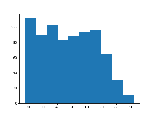
Now let’s have a look at the distribution of ages for the Remain voters:
>>> plt.hist(remainers['age'])
(...)
How about the ages of the Brexiteers?
>>> plt.hist(brexiteers['age'])
(...)
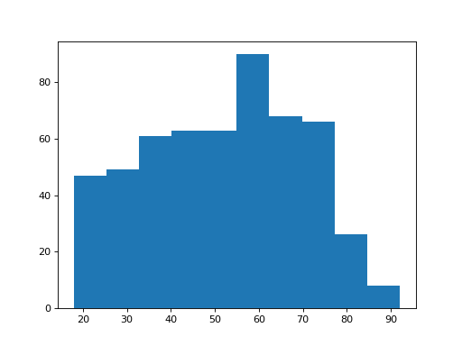
These distributions look different. But — how different are they? And how confident can we be that this difference did not come about by chance?
Last, we will save the data to use it later. First we stack the Remain and Leave cases together into one long data frame:
>>> remain_leave = pd.concat([remainers, brexiteers])
>>> len(remain_leave)
1315
Next we save to a simple text file so we can load it later. The format is CSV, which stands for Comma Separated Values — commas separate the values within each row. In saving, we drop off the first implicit column, with the case numbers:
>>> remain_leave.to_csv('remain_leave.csv', index=False)
To be safe, we check we can load back that file:
>>> remain_leave_reloaded = pd.read_csv('remain_leave.csv')
>>> remain_leave_reloaded
      age  brexit
0      37       1
1      55       1
2      37       1
3      42       1
4      69       1
5      20       1
...

[1315 rows x 2 columns]