\(\newcommand{L}[1]{\| #1 \|}\newcommand{VL}[1]{\L{ \vec{#1} }}\newcommand{R}[1]{\operatorname{Re}\,(#1)}\newcommand{I}[1]{\operatorname{Im}\, (#1)}\)
Comparing two groups with permutation testing
We return to the Brexit age data from Analyzing Brexit.
Here’s the data from the processing we did in Analyzing Brexit:
Download the data file from the link above if you haven’t already got it in your Notebook directory.
>>> import pandas as pd
>>> remain_leave = pd.read_csv('remain_leave.csv')
>>> remainers = remain_leave[remain_leave['brexit'] == 1]
>>> brexiteers = remain_leave[remain_leave['brexit'] == 2]
>>> # Confirm our proportions haven't changed
>>> len(brexiteers) / (len(brexiteers) + len(remainers))
0.4114068441064639
For convenience we get our ages scores into lists for each group:
>>> # We make a list from the Pandas column with the "list" function
>>> brexit_ages = list(brexiteers['age'])
>>> remain_ages = list(remainers['age'])
>>> # Check our proportions again
>>> len(brexit_ages) / (len(brexit_ages) + len(remain_ages))
0.4114068441064639
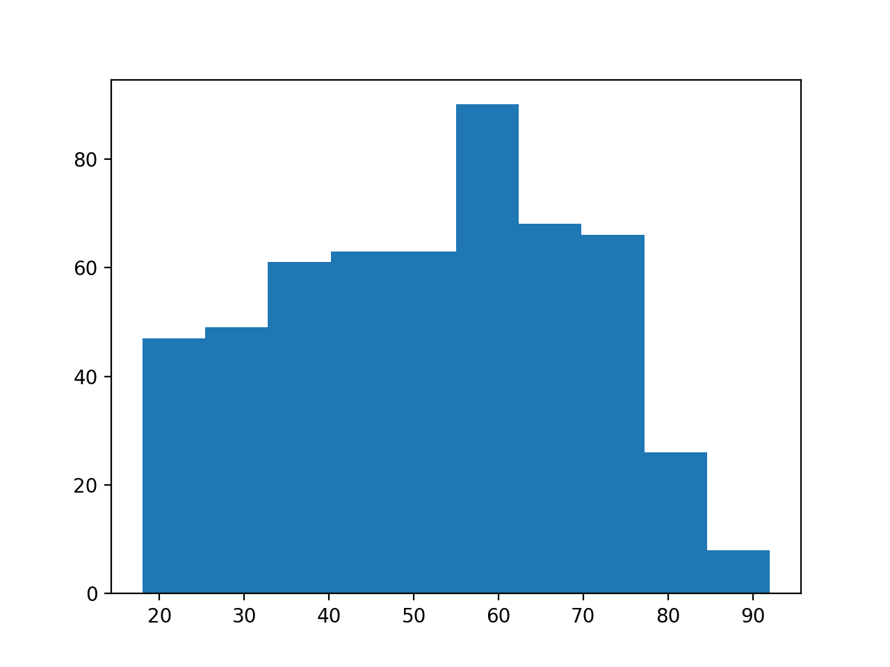
Let’s put up the histograms of these two groups again:
Hint
If running in the IPython console, consider running %matplotlib to enable
interactive plots. If running in the Jupyter Notebook, use %matplotlib
inline.
>>> import matplotlib.pyplot as plt
>>> plt.hist(brexit_ages)
(...)

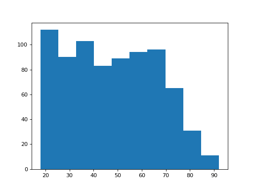
>>> plt.hist(remain_ages)
(...)

The remainers look as though they may be a bit younger on average.
Let’s look at the mean age for the two groups.
The mean of the values in the list is defined as the sum divided by the number of items. Here is the mean age of the Brexit Leave voters:
>>> sum(brexit_ages) / len(brexit_ages)
51.715341959334566
We can define a function to calculate the mean:
>>> def mean(some_list):
...     # Calculates the mean of the values in `some_list`
...     return sum(some_list) / len(some_list)
Now we can get the mean with:
>>> mean(brexit_ages)
51.715341959334566
The mean is lower for the Remain group:
>>> mean(remain_ages)
48.015503875968989
The difference between the means is:
>>> observed_difference = mean(brexit_ages) - mean(remain_ages)
>>> observed_difference
3.6998380833655773
We see that the means of the two groups are different - but can we be confident that this difference did not come about by chance?
What do we mean by chance? Now we have to define our null hypothesis.
We hypothesize that there is in fact no difference between the ages of the two groups. We propose that the difference between the means we see could reasonably occur if we did the following procedure:
- sample 541 + 774 = 1315 people from this same underlying doesn’t-matter-what-you-voted population;
- arbitrarily split this sample into a group of 541 and a group of 774, call
these
group_Aandgroup_B; - calculate the mean age for
group_Aand subtract the mean age ofgroup_B;
Call this procedure - one trial. To test our null hypothesis, we would like to repeat this trial many times, recording the difference in means for each trial. By doing this we could build up a distribution of the kind of differences we would expect by chance - the sampling distribution.
But - we don’t have any more data - so we don’t have many new groups of 541 + 774 = 1315 to sample. But it turns out, we can use the data we have to build the distribution we need.
Let’s start with the null hypothesis - that there is no difference in the ages
of the Leave and Remain groups. If that hypothesis is true, then all the
ages in brexit_ages and in remain_ages can be considered as
being samples from the same underlying group.
To express this, I’m going to pool all the weights into one big group, like this:
>>> # The + below appends the second list to the first
>>> all_ages = brexit_ages + remain_ages
>>> len(all_ages)
1315
In this new pooled list, the first 541 ages are from the brexit_ages list,
and the rest are from the remain_ages list.
Now we have the new pooled list, we can do something similar to taking the new
group_A and group_B groups we imagined above. That is, we can
shuffle the combined group to a random order, and split this shuffled
combined group into a group of 541 and a group of 774. We get the difference
in means of these two groups, and store it. We keep shuffling, to create more
group_A and group_B groups, and more differences in means. The
generated distribution of the mean differences is the distribution we expect
on the null hypothesis, that there is no real difference between the two
groups. We can see where observed_difference lies in this generated
distribution, and this gives us a measure of whether the
observed_difference is likely on the null hypothesis.
Python’s random.shuffle function can do the shuffle for us (see:
Shuffling list element order):
>>> import random
Before shuffling, the first 541 age values are all for Leave voters. Here are the first 10:
>>> # The first 10 ages before shuffling (all brexit)
>>> all_ages[:10]
[71, 60, 74, 61, 47, 56, 76, 35, 44, 38]
Here’s a random shuffle of the combined list of ages:
>>> random.shuffle(all_ages)
>>> # The first 10 ages of the shuffled list, mixed brexit and remain.
>>> all_ages[:10]
[24, 59, 55, 31, 89, 66, 64, 35, 28, 41]
Now for our permutation test. We’ve assumed the null hypothesis. We have
randomly shuffled the combined group. We’ll call the first 541 values
group_A and the last 774 values group_B.
After the shuffling, the group_A group is a random mix of the
brexit_ages and remain_ages values, as is the group_B group.
Here is a function that takes the combined list and returns the difference in means:
>>> def difference_in_means(combined_list):
...     """ Split suffled combind group into two, return mean difference
...     """
...     group_A = combined_list[:541]
...     group_B = combined_list[541:]
...     return mean(group_B) - mean(group_A)
Let’s get the difference in means for these new groups, generated by the shuffle:
>>> difference_in_means(all_ages)
0.35758261808212666
That difference from the shuffled groups looks a lot less than the difference we originally found:
>>> observed_difference
3.6998380833655773
One difference is not enough. We need more shuffled mean differences to see
whether observed_difference is really unusual compared to the range of
permuted group differences. Here we run the shuffle procedure 10000 times, to
get a large range of values:
>>> n_repeats = 10000
>>> shuffled_differences = []  # An empty list to store the differences
>>> for i in range(n_repeats):
...     random.shuffle(all_ages)
...     new_difference = difference_in_means(all_ages)
...     # Collect the new mean by adding to the end of the list
...     shuffled_differences.append(new_difference)
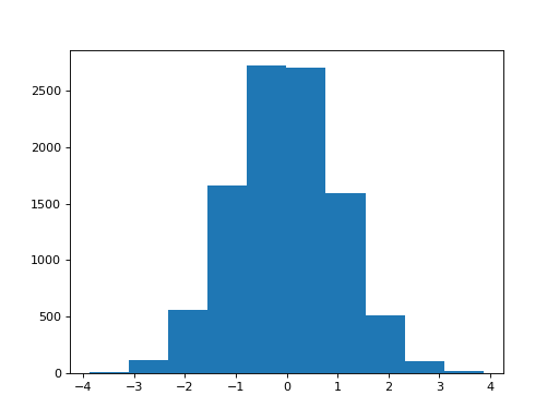
This gives us 10000 differences from groups that are compatible with our null
hypothesis. We can now ask whether observed_difference is unusually
large compared to the distribution of these 10000 differences.
Hint
If running in the IPython console, consider running %matplotlib to enable
interactive plots. If running in the Jupyter Notebook, use %matplotlib
inline.
>>> # The plotting package
>>> import matplotlib.pyplot as plt
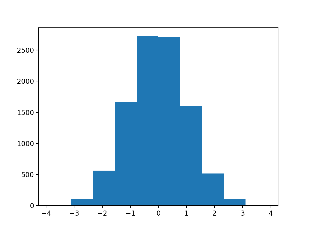
>>> plt.hist(shuffled_differences)
(...)

The maximumum of these differences is:
>>> max(shuffled_differences)
3.8717109191037764
Remember our observed_difference?
>>> observed_difference
3.6998380833655773
So - how many of the shuffled_differences are greater than or equal to the
observed_difference?
>>> n_greater_equal = 0
>>> for i in range(n_repeats):
...     if shuffled_differences[i] >= observed_difference:
...         n_greater_equal = n_greater_equal + 1
>>> n_greater_equal
1
In 10000 samples, we only found one sample greater than or equal to the observed difference.
So, our estimate is that there is a 1 in 10000 chance that the observed difference could have come about by differences in random sampling.