\(\newcommand{L}[1]{\| #1 \|}\newcommand{VL}[1]{\L{ \vec{#1} }}\newcommand{R}[1]{\operatorname{Re}\,(#1)}\newcommand{I}[1]{\operatorname{Im}\, (#1)}\)
Spread of a distribution with number of samples
Have a look back at Testing Brexit Proportions. We found that our sampling distribution of 1315 simulated voters with p=0.519 of voting Brexit was not compatible with the survey proportion of 0.41.
We’re going to be doing some plots, so we start of by getting the plotting libraries:
Hint
If running in the IPython console, consider running %matplotlib to enable
interactive plots. If running in the Jupyter Notebook, use %matplotlib
inline.
>>> #: The stuff you need for plotting a histogram
>>> import matplotlib.pyplot as plt
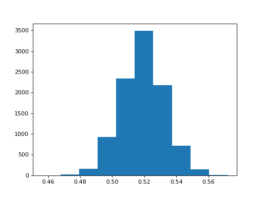
Let’s have a look again at the sampling distribution:
>>> #: The random module
>>> import random
>>> #: function to return a Leave or Remain voter
>>> def leave_or_remain():
...     # Return 1 for Leave, 0 for Remain
...     random_no = random.random()
...     if random_no < 0.519:
...         our_result = 1
...     else:
...         our_result = 0
...     return our_result
Here we get 1315 voters, and calculate a statistic, the proportion of Brexit voters:
>>> #: The statistic value from a single trial
>>> def one_proportion():
...     votes = []
...     for i in range(1315):
...         vote = leave_or_remain()
...         votes.append(vote)
...     brexits = sum(votes)
...     return brexits / len(votes)
Now we want the sampling distribution of this proportion:
>>> n_trials = 10000
>>> proportions = []
>>> for i in range(n_trials):
...     proportion = one_proportion()
...     proportions.append(proportion)
Plot the histogram of the sampling distribution you have just collected:
>>> #- plot the histogram of the sampling distribution
>>> plt.hist(proportions)
(...)

Now - go back to one_proportion above, and change 1315 to 20. Plot the
sampling distribution again, by running the cells above. What do you see?
Try 50, 100 and 1000 instead of 20.