I am going to try and formalize a version of R‘s formula
distinguishing between numeric and factor-like
variables with the distinction that, for a
numeric variable  unlike
in R. It also will not have a ‘’-‘’ operation.
unlike
in R. It also will not have a ‘’-‘’ operation.
A factor is a categorical variable, and the usual interpretation of
> a=factor(levels=c(2,3,4))
> b=factor(levels=c(3,4))
> ~a*b
~a * b
is as the Cartesian product of the columns of indicator matrices for a and b. But in R the formula has meaning even not knowing the levels of a and b. The expression ‘’‘a*b’‘’ above has a multiplication in it. R uses two different multiplications, I will only use one, and it corresponds to R‘s symbol :.
Formally, let  be a set of factors.
Multiplication automatically suggests some algebraic rules
for formulae. We usually think of
factors as obeying the rules
be a set of factors.
Multiplication automatically suggests some algebraic rules
for formulae. We usually think of
factors as obeying the rules
The rules correspond to: idempotency, associativity and commutativity.
If we added an inverse to multiplication, then the set of factors
would constitute a group.
However,
there is no inverse to multiplication. Algebraically,
this means that the set of factors,
combined with this operation and the properties above generates an
algebraic object known as a monoid.
Note, the  above is not the constant 1, but the identity
in the monoid
above is not the constant 1, but the identity
in the monoid  generated by
  and the
product “
and the
product “ “.
Algebraically, this idempotent, commutative monoid is
isomorphic to the join-semilattice
of subsets of with join representing union.
In this view, corresponds to the emptyset
“.
Algebraically, this idempotent, commutative monoid is
isomorphic to the join-semilattice
of subsets of with join representing union.
In this view, corresponds to the emptyset  .
.
In R‘s formulae there is also an addition operation, +. A monoid does not have addition, it only has one operation, multiplication. In order to introduce addition, we need to introduce something like an algebra. If we had a group, the natural structure to consider is called a group algebra or group ring. The corresponding notion for a monoid is that of a monoid ring or a monoid algebra, if the ring used in constructing the monoid ring is commutative. The monoid algebra is constructed from a monoid, which we already have, and a commutative ring.
For the classical ANOVA models (no numeric variables),
we can take this ring to be  .
Below, when
we introduce things like numeric vectors in R
to our formula, we will
change the ring to be the ring of real-valued functions
on some space.
.
Below, when
we introduce things like numeric vectors in R
to our formula, we will
change the ring to be the ring of real-valued functions
on some space.
The monoid algebra  of our monoid over
can be expressed in terms of sets of 2-tuples
of our monoid over
can be expressed in terms of sets of 2-tuples  with multiplication, addition and subtraction defined
as:
with multiplication, addition and subtraction defined
as:
If we introduce variables  then these rules can
be written as
then these rules can
be written as
As our monoid is idempotent and commutative, we arrive at the conclusion that
This places R‘s convention
> a*a
logical(0)
Warning message:
In Ops.factor(a, a) : * not meaningful for factors
into a meaningful algebraic setting.
Actually, R does this for numeric variables as well, unless one uses the I notation.
> terms(formula(~x^2))
~x^2
attr(,"variables")
list(x)
attr(,"factors")
  x
x 1
attr(,"term.labels")
[1] "x"
attr(,"order")
[1] 1
attr(,"intercept")
[1] 1
attr(,"response")
[1] 0
attr(,".Environment")
<environment: R_GlobalEnv>
> terms(formula(~I(x^2)))
~I(x^2)
attr(,"variables")
list(I(x^2))
attr(,"factors")
       I(x^2)
I(x^2)      1
attr(,"term.labels")
[1] "I(x^2)"
attr(,"order")
[1] 1
attr(,"intercept")
[1] 1
attr(,"response")
[1] 0
attr(,".Environment")
<environment: R_GlobalEnv>
Unfortunately, we cannot make sense
of R‘s convention that  in the monoid algebra.
There are a few things wrong with the expression
in the monoid algebra.
There are a few things wrong with the expression  if we take
  to be elements of the monoid .
The most important thing is to note that is not an element
of the algebra , which is the structure where we have
defined addition.
However, we can define an equivalence relation
to be elements of the monoid .
The most important thing is to note that is not an element
of the algebra , which is the structure where we have
defined addition.
However, we can define an equivalence relation
 on as follows
Let the map to equivalence classes be denoted by  . Then,
R‘s convention is equivalent to
. Then,
R‘s convention is equivalent to

or

The set of equivalence classes has a well-defined notion
of addition. Given two equivalence classes  we define

where  is a generic element of the equivalence
class
is a generic element of the equivalence
class  . Since our algebra is an algebra over ,
we can take the generic elements to be random integers, say in the range
[-1e6,1e6]. This means that this notion of the
sum of equivalence classes will break
down occasionally, in the sense
that, with probability roughly 4e-12,
. Since our algebra is an algebra over ,
we can take the generic elements to be random integers, say in the range
[-1e6,1e6]. This means that this notion of the
sum of equivalence classes will break
down occasionally, in the sense
that, with probability roughly 4e-12,  .
In the implementation of this in nipy, the ring we take can be thought of
as the ring of sympy dummy symbols, so, up to memory errors,
.
In the implementation of this in nipy, the ring we take can be thought of
as the ring of sympy dummy symbols, so, up to memory errors,
 always.
The set of equivalence classes  also has a well
defined notion of product
also has a well
defined notion of product
This, too, may occasionally break down depending on how
we define our generic element . If we take
the ring to be  and generate a generic element
by drawing from a random variable with a continuous density, like the
standard normal
and generate a generic element
by drawing from a random variable with a continuous density, like the
standard normal  , then with probability 1, the rules
of addition and multiplication will not break down if we perform
countably many such operations.
, then with probability 1, the rules
of addition and multiplication will not break down if we perform
countably many such operations.
It is not hard to see that the multiplication and addition
are associative, commutative and distributive on .
While addition and multiplication are well-defined on the set of equivalence classes, there is no corresponding notion of subtraction of equivalence classes because, generically,

Therefore, we cannot call the set of equivalence classes a ring
or any other familiar object. As our set of equivalence classes
is just we can delete
the terms from  that appear in
by the elementwise multiplication
that appear in
by the elementwise multiplication

Or, regarding  as subsets of , deletion
of terms is just the operation
as subsets of , deletion
of terms is just the operation  .
.
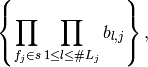
We have now given a formal way of describing which sets of
factors are to be included in a regression model.
The set of factors to be included in a regression model
is specified by an element of where
the monoid is the semilattice of subsets of :math:{cal F}.
On the set of factor specifications , we have
defined two operations that obey the commutative, distributive
and associative properties.
Above, we described rules for specifying which factors are to be included in the model. One can take the same approach for numeric variables, which is essentially what R does. However, R ultimately treats numeric and factors differently when it comes to building the design matrix. For instance,
In the first model below, subtracting 1 yields fitted values orthogonal to the constant, while this is not true in the second model.
> x = rnorm(40)
> y = rnorm(40)
> f = factor(rep(c(1,2),20))

> r1 = resid(lm(y~f-1))
> print(sum(r1))
[1] 1.124101e-15
> r2 = resid(lm(y~x-1))
> print(sum(r2))
[1] 2.616077
There is a perfectly good explanation for this if one uses
R‘s rules for constructing a design matrix
from an element of , as we will see below.
However, it does mean that factors and numerics are treated separately. One way to address this is to consider the monoid

where  is a monoid
for factors that is essentially the same monoid we
saw in the previous section
and
is a monoid
for factors that is essentially the same monoid we
saw in the previous section
and  is a monoid for numerical variables. The multiplication in this monoid is defined componentwise

The only remaining issue is how do we define multiplication in the monoid
. R uses the same idempotency rules as for factors,
though it seems more natural to use true multiplication instead.
> lm(y~x*x)$coef
 (Intercept)            x
0.0775913698 0.0003296236
> lm(y~x)$coef
 (Intercept)            x
0.0775913698 0.0003296236
This leaves room for some weird manipulations
> lm(y~x*log(exp(x)))

Call:
lm(formula = y ~ x * log(exp(x)))

Coefficients:
  (Intercept)              x    log(exp(x))  x:log(exp(x))
      0.06966        0.01130             NA        0.01779

> lm(y~x + I(x^2))

Call:
lm(formula = y ~ x + I(x^2))

Coefficients:
(Intercept)            x       I(x^2)
    0.06966      0.01130      0.01779
Using a symbolic system, like sympy can be helpful in cases like this.
Before continuing,
let us make a slight modification of the previous monoid
that recognizes the fact that these objects
are meant to represent random variables, that is functions on some
sample space  . The process of constructing the
design matrix is then just the evaluation of these functions
at some point
. The process of constructing the
design matrix is then just the evaluation of these functions
at some point  . If we want to think
of a more concrete probability model, we can think
of a data.frame with
. If we want to think
of a more concrete probability model, we can think
of a data.frame with  rows as a point in
  and our probability distribution might correspond to IID samples
from some probability measure
and our probability distribution might correspond to IID samples
from some probability measure  .
Of course, constructing the design matrix is completely
separate from specifying the joint distribution on , but
thinking of factors and numeric variables as functions
makes things more concrete.
.
Of course, constructing the design matrix is completely
separate from specifying the joint distribution on , but
thinking of factors and numeric variables as functions
makes things more concrete.
In this new view, a factor from the previous section is now defined as a
function  where
where  is the set of
levels of the factor. We define a numeric variable as a real-valued function
on .
is the set of
levels of the factor. We define a numeric variable as a real-valued function
on .
With this definition, is a (finite) collection of functions
on , each taking values in a different space, and
is the same monoid as before. Therefore,
a member of the set of equivalence classes  can be viewed as a set of functions
We might then take  to be the monoid
of real-valued functions on with multiplication
defined in the obvious way
to be the monoid
of real-valued functions on with multiplication
defined in the obvious way

There is, however, a possible measure theoretic
complication to consider as we should properly consider
equivalence classes on  defined
by equality up to sets of probability 0 according to some
probability space .
Let us therefore fix this probability space
and take
defined
by equality up to sets of probability 0 according to some
probability space .
Let us therefore fix this probability space
and take  ,
the collection of random variables on .
,
the collection of random variables on .
Carrying out the same construction of equivalence classes
as for factors, our model is represented as a member of
 .
Viewing this as a subset, our model is
.
Viewing this as a subset, our model is

Hence, our model is a collection of tuples of real-valued random variables
combined with a subset of the factors , each
of which are also functions defined on .
Given a description of our model, i.e. a set of tuples

we now must build a design matrix.
Formally, this corresponds to constructing a function
 from
from  ,
and then evaluating this function at a
point
,
and then evaluating this function at a
point  which yields a matrix
Part of the construction is also to determine
a well-defined set of names for each column of  .
.
Given a linear, or total ordering on the random variables
we see in , i.e.
the process of building this design matrix can
be carried out in stages based on the functions  .
Let the ordering be determined as
.
Let the ordering be determined as  .
For each
.
For each  , we construct a function
 and the final function is determined by
concatenation in the order previously determined
and the final function is determined by
concatenation in the order previously determined

where the multiplication above is elementwise.
In R this linear ordering seems to be based on the name of the variable in the expression, with 1, the intercept coming before all others
> z = rnorm(40)
> lm(y~x+z)$coef
  (Intercept)             x             z
 0.0429108507 -0.0007459873 -0.1763908600
> b = x
> a = z
> lm(y~a+b)$coef
  (Intercept)             a             b
 0.0429108507 -0.1763908600 -0.0007459873
> lm(y~(x+z)*f)$coef
(Intercept)           x           z          f2        x:f2        z:f2
  0.2353311   0.5266701  -0.7416684  -0.2650608  -0.4068248   0.9817334
> lm(y~(a+b)*f)$coef
(Intercept)           a           b          f2        a:f2        b:f2
  0.2353311  -0.7416684   0.5266701  -0.2650608   0.9817334  -0.4068248
To construct the coding of the factors, R uses rules as described in Hastie & Chambers (1988) meant to satisfy users expectations in common statistical settings. For instance, in the case of two factors with one nested in the other, this rule produces the “expected result”.
In our notation, constructing this matrix is equivalent to constructing
a function . Here,
 is the number of real-valued functions, i.e. random variables, specified by which
may be viewed as a collection of subsets of .
is the number of real-valued functions, i.e. random variables, specified by which
may be viewed as a collection of subsets of .
The collection of subsets of is naturally graded, i.e.
can be partially ordered in terms of the size of each subset on
. Let  represent this
ordering where each
represent this
ordering where each  and,
possibly,
and,
possibly,  . Now, each
  will contribute a
certain number of random variables to
will contribute a
certain number of random variables to  that are concatenated
together. The number of random variables depends on how each factor
that are concatenated
together. The number of random variables depends on how each factor  is coded. The coding of a factor
  is defined as a choice
of a random vector
is defined as a choice
of a random vector  . The types
of coding fall into two groups either indicator or contrast. If a factor is
coded with indicator variables, then
. The types
of coding fall into two groups either indicator or contrast. If a factor is
coded with indicator variables, then  , the number of
levels of . If a factor is coded with contrast variables, then
, the number of
levels of . If a factor is coded with contrast variables, then
 .
.
For each factor , and a linear ordering of  we can define
  binary random
variables
binary random
variables
An indicator coding is any set of functions whose linear span
coincides with the linear span of  . Usually,
these functions are just taken to be the
. Usually,
these functions are just taken to be the  ‘s themselves.
A contrast coding is a set of  independent linear
combinations of the chosen in various ways, each with different
interpretations.
independent linear
combinations of the chosen in various ways, each with different
interpretations.
> t(contr.helmert(4))
      1  2  3 4
[1,] -1  1  0 0
[2,] -1 -1  2 0
[3,] -1 -1 -1 3
> t(contr.poly(4))
         [,1]       [,2]       [,3]      [,4]
.L -0.6708204 -0.2236068  0.2236068 0.6708204
.Q  0.5000000 -0.5000000 -0.5000000 0.5000000
.C -0.2236068  0.6708204 -0.6708204 0.2236068
> t(contr.sum(4))
     1 2 3  4
[1,] 1 0 0 -1
[2,] 0 1 0 -1
[3,] 0 0 1 -1
> t(contr.treatment(4))
  1 2 3 4
2 0 1 0 0
3 0 0 1 0
4 0 0 0 1
> t(contr.SAS(4))
  1 2 3 4
1 1 0 0 0
2 0 1 0 0
3 0 0 1 0
For instance, contr.sum (which corresponds to nipy‘s main_effect) uses the random variables

The rule R uses to construct the codings for
a given  produces a set of random
variables whose linear span is equivalent to the linear span of
produces a set of random
variables whose linear span is equivalent to the linear span of
The way it produces these columns depends on a linear
ordering of . Let 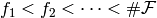 be this linear ordering. This, in turn, determines a linear ordering
on all subsets of . Note that this linear ordering
corresponds to
representing sets as sorted tuples, so that
is a sorted list of sorted tuples.
be this linear ordering. This, in turn, determines a linear ordering
on all subsets of . Note that this linear ordering
corresponds to
representing sets as sorted tuples, so that
is a sorted list of sorted tuples.
We therefore now assume that has been linearly ordered
as 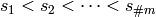 .
.
This next step is a bit of a mouthful, but, here goes
for any  , the linear span of the random variables
is equivalent to the linear span of
In words, the linear space spanned by using the indicator coding
for each factor in is equivalent to the column
space spanned by using the contrast coding
for each  and concatenating
them all together.
and concatenating
them all together.
Hence, the column space spanned by using the indicator coding
for each factor in both of  is equivalent
to using the contrast coding for each factor in
every subset
is equivalent
to using the contrast coding for each factor in
every subset  or
or  . The collection of such subsets forms an abstract
simplicial complex with maximal simplices
. The collection of such subsets forms an abstract
simplicial complex with maximal simplices  .
.
R effectively constructs the function sequentially,
based on stages  in such a way that, for each
  , the linear span of the coordinate
functions of of
, the linear span of the coordinate
functions of of  is the same as the linear span of
using all indicator codings for each factor in each of the subsets
is the same as the linear span of
using all indicator codings for each factor in each of the subsets ![[s_1,\dots, s_i]](_images/math/fce47c6ee09ec8f08e2c95124810118697bffa89.png) .
.
By construction, then, the coordinate functions of the final function  span the same space as if it has used the indicator
codings for each factor in each of the
span the same space as if it has used the indicator
codings for each factor in each of the ![[s_1, \dots, s_{\# m}]](_images/math/94ba377f1c42b8e0f6c3dd7a4b37d48a8d3c9ad0.png) .
.
The rule can be expressed in terms of operations on simplicial complexes:
def factor_codings(*factor_monomials):
    """ Find which factors to code with indicator or contrast variables

    Determine which factors to code with indicator variables (using
    len(factor.levels) columns of 0s and 1s) or contrast coding (using
    len(factor.levels)-1).  The elements of the sequence should be tuples of
    strings.  Further, the factors are assumed to be in *graded* order, that is
    [len(f) for f in factor_monomials] is assumed non-decreasing.

    Examples
    --------
    >>> factor_codings(('b',), ('a',), ('b', 'c'), ('a','b','c'))
    {('b', 'c'): [('b', 'indicator'), ('c', 'contrast')], ('a',): [('a', 'contrast')], ('b',): [('b', 'indicator')], ('a', 'b', 'c'): [('a', 'contrast'), ('b', 'indicator'), ('c', 'indicator')]}
    >>> factor_codings(('a',), ('b',), ('b', 'c'), ('a','b','c'))
    {('b', 'c'): [('b', 'indicator'), ('c', 'contrast')], ('a',): [('a', 'indicator')], ('b',): [('b', 'contrast')], ('a', 'b', 'c'): [('a', 'contrast'), ('b', 'indicator'), ('c', 'indicator')]}

    Here is a version with debug strings to see what is happening:

    >>> factor_codings(('a',), ('b', 'c'), ('a','b','c')) #doctest: +SKIP
    Adding a from ('a',) as indicator because we have not seen any factors yet.
    Adding b from ('b', 'c') as indicator because set([('c',), ()]) is not a subset of set([(), ('a',)])
    Adding c from ('b', 'c') as indicator because set([(), ('b',)]) is not a subset of set([(), ('a',)])
    Adding a from ('a', 'b', 'c') as contrast because set([('c',), ('b', 'c'), (), ('b',)]) is a subset of set([('b', 'c'), (), ('c',), ('b',), ('a',)])
    Adding b from ('a', 'b', 'c') as indicator because set([('c',), (), ('a', 'c'), ('a',)]) is not a subset of set([('b', 'c'), (), ('c',), ('b',), ('a',)])
    Adding c from ('a', 'b', 'c') as indicator because set([('a', 'b'), (), ('b',), ('a',)]) is not a subset of set([('b', 'c'), (), ('c',), ('b',), ('a',)])
    {('b', 'c'): [('b', 'indicator'), ('c', 'indicator')], ('a',): [('a', 'indicator')], ('a', 'b', 'c'): [('a', 'contrast'), ('b', 'indicator'), ('c', 'indicator')]}

    Notes
    -----
    Even though the elements of factor_monomials are assumed to be in graded
    order, the final result depends on the ordering of the strings of the
    factors within each of the tuples.
    """
    lmax = 0
    from copy import copy
    already_seen = set([])
    final_result = []
    for factor_monomial in factor_monomials:
        result = []
        factor_monomial = list(factor_monomial)
        if len(factor_monomial) < lmax:
            raise ValueError('factors are assumed to be in graded order')
        lmax = len(factor_monomial)

        for j in range(len(factor_monomial)):
            cur = copy(list(factor_monomial))
            cur.pop(j)
            terms = simplicial_complex(cur)[2]
            if already_seen and set(terms).issubset(already_seen):
                result.append((factor_monomial[j], 'contrast'))
            else:
                result.append((factor_monomial[j], 'indicator'))
        already_seen = already_seen.union(simplicial_complex(factor_monomial)[2])
        final_result.append((tuple(factor_monomial), result))
    return dict(final_result)
These types of expressions are used in R to construct design matrices.
> c = factor(levels=c('warm', 'hot'))
> a + a:b + b:c + a:b:c
Error in b:c : NA/NaN argument
In addition: Warning messages:
1: In a:b : numerical expression has 40 elements: only the first used
2: In a:b : numerical expression has 40 elements: only the first used
3: In b:c : numerical expression has 40 elements: only the first used
I
However, R does not meaningfully handle this product. In order to construct a design matrix, R tries to come up with a smart parameterization of all the columns represented in the formula above. Note also that I overwrote c, one of R‘s most fundamental objects, oops.
Here is an example where the product is made sense of and used in a linear model.
> a = factor(rep(c(1,1,1,1,2,2,2,2,3,3,3,3), 10))
> b = factor(rep(c(1,1,2,2,1,1,2,2,1,1,2,2),10))
> cc = factor(rep(c('hot','warm','hot','warm','hot','warm','hot','warm','hot'
,'warm','hot','warm'),10))
> Y = rnorm(120)

> lm1 = lm(Y~a+b+cc+a:b:cc-1)
> print(lm1$coef)
          a1           a2           a3           b2       ccwarm  a1:b1:cchot
  -2.2061381   -2.2196141   -1.2529329    1.0173781    1.0550321    2.1112981
 a2:b1:cchot  a3:b1:cchot  a1:b2:cchot  a2:b2:cchot  a3:b2:cchot a1:b1:ccwarm
   1.5869000    1.3813130    0.8630796    1.2249425           NA    0.8034864
a2:b1:ccwarm a3:b1:ccwarm a1:b2:ccwarm a2:b2:ccwarm a3:b2:ccwarm
   1.1049333           NA           NA           NA           NA
At this point, the algebraic tools being used are slightly different. The
monoid structure is forgotten and we turn to working with simple polynomials.
What R does is tries to find an alternative, but equivalent, expression for
something like  because it recognizes
  as maximal in the formula above even though
  as well as
 and
and  also appear. In this case, equivalence
means equivalence in the additive sense. That is, it constructs a second element
of this monoid ring such that the column span, when computed, is identical to
that of which is the pairwise product of the dummy
indicator variables
also appear. In this case, equivalence
means equivalence in the additive sense. That is, it constructs a second element
of this monoid ring such that the column span, when computed, is identical to
that of which is the pairwise product of the dummy
indicator variables  . The polynomials that R uses for this are
generated by
. The polynomials that R uses for this are
generated by  . An expression of
the form
. An expression of
the form  indicates that R will use “contrasts” instead of
“dummy variables” to encode this factor in the expression. There are several
choices of contrast to use.
indicates that R will use “contrasts” instead of
“dummy variables” to encode this factor in the expression. There are several
choices of contrast to use.
If the contrast encoding involves dropping a term, say, the term corresponding to the last level in a factor, then the expression
has columns
[a_2 * b_3 * c_hot, a_2 * b_4 * c_hot]
Note that this assumes an ordering of the levels of a factor. This is not a problem, but it makes some difference in terms of what columns of the design matrix are produced by R. For instance, if we changed “hot” to “S” for “sweltering” and “warm” to “C” for “comfy” in the levels of c then the design matrix would have columns
[a_2 * b_3 * c_C, a_2 * b_4 * c_C]
Therfore, the columns that R generates depend on the order of the levels of the factors, and we will see, they also depend on the order of the names of the factors.
> dd = factor(rep(c('S','C','S','C','S','C','S','C','S','C','S','C'),10))

> lm2 = lm(Y~a+b+dd+a:b:dd-1)
> print(lm2$coef)
        a1         a2         a3         b2        ddS  a1:b1:ddC  a2:b1:ddC
 1.0932867  1.4416736  1.1834122 -0.3639349 -1.0550321 -1.4409063 -1.5013222
 a3:b1:ddC  a1:b2:ddC  a2:b2:ddC  a3:b2:ddC  a1:b1:ddS  a2:b1:ddS  a3:b1:ddS
-1.3813130 -0.8630796 -1.2249425         NA -0.1330946 -1.0193555         NA
 a1:b2:ddS  a2:b2:ddS  a3:b2:ddS
        NA         NA         NA

> print(sum((fitted(lm1)-fitted(lm2))^2))
[1] 2.20623e-29
The point of these code snippets is to emphasize that the columns created by R depend on a total linear ordering of monomials whose names depend both on the factor names and the factor levels. Algebraically, the monomial
knows nothing about the levels of the factors so it
does not know how to construct this design matrix. However,
we can create a linear ordering of the
monomials given a linear ordering of .
The algorithm R uses to construct the columns of the design matrix is
relatively straightforward, at least as described in Hastie & Chambers (1992),
once the linear ordering of the monomials in the monoid ring is fixed, as well
as the ordering of the levels of the factors. As the monoid ring is graded
graded, there is a natural
ordering of monomials in terms of the cardinality of the subsets they represent
(remember our monoid ring is algebraically isomorphic to the semi-lattice of
subsets of with binary opertion  ). This is just to
emphasize that to implement R‘s algorithm, we must specify a total ordering
within monomials of a fixed degree. R seems to use the name of the factor to
create this ordering.
). This is just to
emphasize that to implement R‘s algorithm, we must specify a total ordering
within monomials of a fixed degree. R seems to use the name of the factor to
create this ordering.
Given a sequence,  of monomials in the monoid ring, R first creates a
new sequence
of monomials in the monoid ring, R first creates a
new sequence  of monomials of the same length as in the
monoid ring such that for each
of monomials of the same length as in the
monoid ring such that for each  , the 'maximal elements' in
![S[:i]](_images/math/c69d46e48312cf190136b4399d288c6bffce408c.png) and
and ![N[:i]](_images/math/87b0c49486f5a0b604da78ca65095dfb78d4fc55.png) are identical. In turn, this means that the
columns of the design matrix generated by and are
identical. Therefore, the design matrix generated by and
have the same column space.
are identical. In turn, this means that the
columns of the design matrix generated by and are
identical. Therefore, the design matrix generated by and
have the same column space.
It then uses this new sequence to ultimately construct the design
matrix. The span of the columns of the design matrix will always include the
span of the dummy encoding of this maximal monomial. Sometimes, it will yield a
full-rank design matrix, and sometimes not.
Given a sequence of monomials in the monoid ring (not necessarily sorted) R‘s is essentially:
N = []
for idx, monomial in enumerate(S):
   new_monomial = 1
   for variable in monomial:
       margin = monomial / variable
       if margin in generated(S[:idx]):
           new_monomial *= (variable - 1)
       else:
           new_monomial *= variable
   N.append(new_monomial)
Formally, this ordering of the ring takes the expression

and yields sorted sequences of orders 0 through 3, in this case. In R‘s version, the sequences are sequences, rather then sets, i.e. the order matters. For our expression above, we have the following sequences:
S[0] = ['']
S[1] = ['a']
S[2] = ['ab','bc']
S[3] = ['abc']

# this gives a linear ordering
initial = S[0] + S[1] + S[2] + S[3]
The algorithm proceeds as
final = []
for i, p in enumerate(initial):
   q = p.copy()
   for s in p:
      q = q.replace(s, '')
      if q in genereated(initial[:i]):
         q = q.replace('(%s-1)' % s, s)
   final.append(q)
final = []
for i, p in enumerate(initial):
   q = p.copy()
   for s in p:
      if q.remove(s) in initial:
         q = q.replace('(%s-1)' % s, s)
   final.append(q)